Parallel Programming Using FastFlow
(Version September 2015)
Massimo Torquati
Computer Science Department, University of Pisa
torquati@di.unipi.it
Summary
Chapter 1
Introduction
FastFlow is an open-source, structured parallel programming framework originally
conceived to support highly efficient stream parallel computation while targeting
shared memory multi-core. Its efficiency comes mainly from the optimised
implementation of the base communication mechanisms and from its layered design.
FastFlow provides the parallel applications programmer with a set of ready-to-use,
parametric algorithmic skeletons modelling the most common parallelism
exploitation patterns. The algorithmic skeletons provided by FastFlow may
be freely nested to model more and more complex parallelism exploitation
patterns.
FastFlow is an algorithmic skeleton programming framework developed and
maintained by the parallel computing group at the Departments of Computer Science
of the Universities of Pisa and Torino [9].
Fig. 1.1 presents a brief history of the algorithmic skeleton programming model.
For a more in-depth description, please refer to [14].
A number of papers and technical reports discuss the different features of this
programming environment [10, 5, 2], the results achieved when parallelizing different
applications [18, 11, 15, 8, 1, 7, 6] and the use of FastFlow as software accelerator,
i.e. as a mechanism suitable for exploiting unused cores of a multi-core architecture
to speed up execution of sequential code [3, 4]. This work represents instead a
tutorial aimed at describing the use of the main FastFlow skeletons and patterns and
its programming techniques, providing a number of simple (and not so simple) usage
examples.
This tutorial describes the basic FastFlow concepts and the main skeletons
targeting stream-parallelism, data-parallelism and data-flow parallelism. It is
still not fully complete: for example important arguments and FastFlow features such
as the FastFlow memory allocator, the thread to core affinity mapping, GPGPU
programming and distributed systems programming are not yet covered in this
tutorial.
Parallel patterns vs parallel skeletons:
Algorithmic skeletons and parallel design patterns have been developed in completely disjoint
research frameworks but with almost the same objective: providing the programmer of parallel
applications with an effective programming environment. The two approaches have many
similarities addressed at different levels of abstraction. Algorithmic skeletons are aimed at
directly providing pre-defned, efficient building blocks for parallel computations to the
application programmer, whereas parallel design patterns are aimed at providing directions,
suggestions, examples and concrete ways to program those building blocks in different
contexts.
We want to emphasise the similarities of these two concepts and so, throughout this tutorial,
we use the terms pattern and skeleton interchangeably. For an in-depth discussion
on the similarities and the main differences of the two approaches please refer to
[14].
This tutorial is organised as follow: Sec. 1.1 describes how to download the
framework and compile programs, Sec. 2 recalls the FastFlow application design
principles. Then, in Sec. 3 we introduce the main features of the stream-based
parallel programming in FastFlow: how to wrap sequential code for handling a steam
of data, how to generate streams and how to combine pipelines, farms and loop
skeletons, how to set up farms and pipelines as software accelerator. In Sec. 4 we
introduce data-parallel computations in FastFlow. ParallelFor, ParallelForReduce,
ParallelForPipeReduce and Map are presented in this section. Finally, in Sec. 5, the
macro data-flow programming model provided by the FastFlow framework is
presented.
1.1 Installation and program compilation
FastFlow is provided as a set of header files. Therefore the installation process is
trivial, as it only requires to download the last version of the FastFlow source code
from the SourceForge (http://sourceforge.net/projects/mc-_fastflow/)
by using svn:
svn co https://svn.code.sf.net/p/mc-fastflow/code fastflow
Once the code has been downloaded (with the above svn command, a fastflow folder
will be created in the current directory), the directory containing the ff
sub-directory with the FastFlow header files should be named in the -I flag of g++,
such that the header files may be correctly found.
For convenience may be useful to set the environment variable FF_ROOT to point
to the FastFlow source directory. For example, if the FastFlow tarball (or the svn
checkout) is extracted into your home directory with the name fastflow, you may
set FF_ROOT as follows (bash syntax):
export FF_ROOT=$HOME/fastflow
Take into account that, since FastFlow is provided as a set of .hpp source files,
the -O3 switch is essential to obtain good performance. Compiling with no -O3
compiler flag will lead to poor performance because the run-time code will not be
optimised by the compiler. Also, remember that the correct compilation
of FastFlow programs requires linking the pthread library (-pthread
flag).
g++ -std=c++11 -I$FF_ROOT -O3 test.cpp -o test -pthread
1.1.1 Tests and examples
In this tutorial a set of simple usage examples and small applications are
described. In almost all cases, the code can be directly copy-pasted into a text
editor and then compiled as described above. For convenience all codes are
provided in a separate tarball file fftutorial_source_code.tgz with a
Makefile.
At the beginning of all tests and examples presented, there is included the file
name containing the code ready to be compiled and executed, for example:
1/* **************************** */ 2/* ******* hello_node.cpp ***** */ 3 4#include <iostream> 5#include <ff/node.hpp> 6using namespace ff; 7struct myNode:ff_node { 8....
means that the above code is in the file hello_node.cpp.
Chapter 2
Design principles
FastFlow has been originally designed to provide programmers with efficient
parallelism exploitation patterns suitable to implement (fine grain) stream parallel
applications. In particular, FastFlow has been designed
- to promote high-level parallel programming, and in particular skeletal
programming (i.e. pattern-based explicit parallel programming), and
- to promote efficient programming of applications for multi-core.
More recently, within the activities of the EU FP7 STREP project
”ParaPhrase”
the FastFlow framework has been extended in several ways. In particular, in the
framework have been added:
- several new high-level patterns
- facilities to support coordinated execution of FastFlow program on
distributed multi-core machines
- support for execution of new data parallel patterns on GPGPUs
- new low-level parallel building blocks allowing to build almost any kind of
streaming graph and parallel patterns.
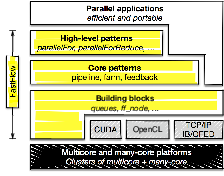
The whole programming framework has been incrementally developed according
to a layered design on top of Pthread/C++ standard programming framework as
sketched in Fig. 2.1).
The Building blocks layer provides the basics blocks to build (and generate via
C++ header-only templates) the run-time support of core patterns. Typical objects
at this level are queues (e.g. lock-free SPSC queues, bounded and unbounded),
process and thread containers (as C++ classes) mediator threads/processes
(extensible and configurable schedulers and gatherers). The shared-memory run-time
support extensively uses non-blocking lock-free algorithms, the distributed run-time
support employs zero-copy messaging, the GPGPUs support exploits asynchrony and
SIMT optimised algorithms.
The Core patterns layer provides a general data-centric parallel programming
model with its run-time support, which is designed to be minimal and reduce to the
minimum typical sources of overheads in parallel programming. At this level there are
two patterns (task-farm and all its variants and pipeline) and one pattern-modifier
(feedback). They make it possible to build very general (deadlock-free) cyclic process
networks. They are not graphs of tasks, they are graphs of parallel executors
(processes/threads). Tasks or data items flows across them according to the
data-flow model. Overall, the programming model can be envisioned as a
shared-memory streaming model, i.e. a shared-memory model equipped with
message-passing synchronisations. They are implemented on top of building
blocks.
The High-level patterns are clearly characterised in a specific usage context
and are targeted to the parallelisation of sequential (legacy) code. Examples are
exploitation of loop parallelism (ParallelFor and its variants), stream parallelism
(pipeline and task-farm), data-parallel algorithms (map, poolEvolution, stencil,
StencilReduce), execution of general workflows of tasks (mdf - Macro Data-Flow),
etc. They are typically equipped with self-optimisation capabilities (e.g.
load-balancing, grain auto-tuning, parallelism-degree auto-tuning) and exhibit
limited nesting capability. Some of them targets specific devices (e.g. GPGPUs).
They are implemented on top of core patterns.
Parallel application programmers are supposed to use FastFlow directly
exploiting the parallel patterns available at the ”High-level” or ”Core” levels. In
particular:
- defining sequential concurrent activities, by sub classing a proper FastFlow
class, the ff_node (or ff_minode and ff_monode) class, and
- building complex stream parallel patterns by hierarchically composing
sequential concurrent activities, pipeline patterns, feedbacks, task-farm
patterns and their ”specialised” versions implementing more complex
parallel patterns.
Concerning the usage of FastFlow to support parallel application development on
shared memory multi-core, the framework provides two possible abstractions of
structured parallel computation:
- a skeleton program abstraction used to implement applications completely
modelled according to the algorithmic skeleton concepts. When using this
abstraction, the programmer writes a parallel application by providing
the business logic code, wrapped into proper ff_node sub-classes, a
skeleton (composition) modelling the parallelism exploitation pattern of
the application and a single command starting the skeleton computation
and awaiting for its termination.
- an accelerator abstraction used to parallelize (and therefore to accelerate)
only some parts of an existing application. In this case, the programmer
provides a skeleton composition which is run on the ”spare” cores of the
architecture and implements a parallel version of part of the business logic
of the application, e.g. the one computing a given f(x). The skeleton
composition, if operating on stream (i.e. pipeline or task-farm based
compositions), will have its own input and output channels. When an
f(xj) has to be computed within the application, rather than writing code
to call to the sequential f code, the programmer may insert asynchronous
”offloading” calls for sending xj to the accelerator skeleton. Later on,
when the result of f(xj) has to be used, the code needed for ”reading”
accelerator results may be used to retrieve the computed values.
This second abstraction fully implements the ”minimal disruption” principle stated by
Cole in his skeleton manifesto [13], as the programmer using the accelerator is only
required to program a couple of offload/get_result primitives in place of the
single … = f(x) function call statement (see Sec. 3.7).
Chapter 3
Stream parallelism
An application may operate on values organised as streams. A stream is a possibly
infinite sequence of values, all of them having the same data type, e.g. a stream of
images (not necessarily all having the same format), a stream of files, a stream of
network packets, a stream of bits, etc.
A complex streaming application may be seen as a graph (or workflow) of
computing modules (sequential or parallels) whose arcs connecting them bring
streams of data of different types. The typical requirements of such a complex
streaming application is to guarantee a given Quality of Service imposed
by the application context. In a nutshell, that means that the modules of
the workflow describing the application have to be able to sustain a given
throughput.
There are many applications in which the input streams are primitive, because
they are generated by external sources (e.g. HW sensors, networks, etc..) or I/O.
However, there are cases in which streams are not primitive, but it is possible that
they can be generated directly within the program. For example, sequential loops or
iterators. In the following we will see how to generate a stream of data in FastFlow
starting from sequential loops.
3.1 Stream parallel skeletons
Stream parallel skeletons are those natively operating on streams, notably pipeline
and task-farm (or simply farm).
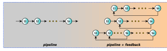
pipeline
The pipeline skeleton is typically used to model computations expressed in stages. In
the general case, a pipeline may have more than two stages, and it can be built as a
single pipeline with N stages or as pipeline of pipelines. Given a stream of input
tasks

the pipeline with stages

computes the output stream

The parallel semantics of the pipeline skeleton ensures that all the stages will be
execute in parallel. It is possible to demonstrate that the total time required to
entirely compute a single task (latency) is close to the sum of the times required to
compute the different stages. And, the time needed to output a new result
(throughput) is close to time spent to compute a single task by the slowest stage in
the pipeline.
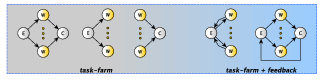
task-farm
The task-farm (sometimes also called master-worker) is a stream parallel paradigm
based on the replication of a purely functional computation. The farm skeleton is
used to model embarrassingly parallel computations. The only functional parameter
of a farm is the function f needed to compute the single task. The function f is
stateless. Only under particular conditions, functions with internal state, may be
used.
Given a stream of input tasks

the farm with function f computes the output stream

Its parallel semantics ensures that it will process tasks such that the single task
latency is close to the time needed to compute the function f sequentially, while the
throughput (only under certain conditions) is close to  where n is the number of
parallel agents used to execute the farm (called workers), i.e. its parallelism
degree.
where n is the number of
parallel agents used to execute the farm (called workers), i.e. its parallelism
degree.
The concurrent scheme of a farm is composed of three distinct parts: the
Emitter, the pool of workers and the Collector. The Emitter gets a farm’s input
tasks and distributes them to workers using a given scheduling strategy. The
Collector collects tasks from workers and sends them to the farm’s output
stream.
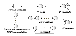
3.2 FastFlow abstractions
In this section we describe the sequential concurrent activities (ff_node,
ff_minode, ff_monode and ff_dnode), and the ”core” skeletons pipeline and
task-farm (see Fig 3.1) used as building blocks to model composition and parallel
executions. The core skeletons are ff_node derived objects as well, so they can be
nested and composed in almost any arbitrary way. The feedback pattern modifier
can also be used in the pipeline and task-farm to build complex cyclic streaming
networks.
3.2.1 ff_node
The ff_node sequential concurrent activity abstraction provides a means to define a
sequential activity (via its svc method) that a) processes data items appearing on a
single input channel and b) delivers the related results onto a single output
channel.
In a multi-core, a ff_node object is implemented as a non-blocking thread
(or a set of non-blocking threads). This means that the number of ff_node(s)
concurrently running should not exceed the number of logical cores of the platform at
hand. The latest version of FastFlow supports also blocking run-time. It is
possible to select the blocking run-time by compiling the code with the flag
-DBLOCKING_MODE.
The ff_node class actually defines a number of methods, the following three
virtual methods are of particular importance:
1public: 2 virtual void* svc(void *task) = 0; // encapsulates user’s business code 3 virtual int svc_init() { return 0; }; // initialization code 4 virtual void svc_end() {} // finalization code
The first is the one defining the behaviour of the node while processing the input
stream data items. The other two methods are automatically invoked once and for all
by the FastFlow RTS when the concurrent activity represented by the node is started
(svc_init) and right before it is terminated (svc_end). These virtual methods
may be overwritten in the user supplied ff_node sub-classes to implement
initialisation code and finalisation code, respectively. Since the svc method is a pure
virtual function, it must be overwritten.
A FastFlow ff_node can be defined as follow:
1#include <ff/node.hpp> 2using namespace ff; 3struct myStage: ff_node { 4 int svc_init() { // not mandatory 5 // initialize the stage 6 return 0; // returing non zero means error! 7 } 8 void *svc(void *task) { 9 // business code here working on the input ’task’ 10 return task; // may return a task or EOS,GO_ON,GO_OUT,EOS_NOFREEZE 11 } 12 void svc_end() { // not mandatory 13 // finalize the stage, free resources,... 14 } 15};
The ff_node behaves as a loop that gets an input task (coming from the input
channel), i.e. the input parameter of the svc method, and produces one or more
outputs, i.e. the return value of the svc method or the invocation of the
ff_send_out method that can be called inside the svc method. The loop
terminates either if the output provided or the input received is a special value:
”End-Of-Stream” (EOS). The EOS is propagated across channels to the next
ff_node.
Particular cases of ff_nodes may be simply implemented with no input channel
or no output channel. The former is used to install a concurrent activity generating
an output stream (e.g. from data items read from keyboard or from a disk file); the
latter to install a concurrent activity consuming an input stream (e.g. to present
results on a video, to store them on disk or to send output packets into the
network).
The simplified life cycle of an ff_node is informally described in the following
pseudo-code:
do {
if (svc_init() < 0) break;
do {
intask = input_stream.get();
if (task == EOS) output_stream.put(EOS);
else {
outtask = svc(intask);
output_stream.put(EOS);
}
} while(outtask != EOS);
svc_end();
termination = true;
if (thread_has_to_be_frozen() == "yes") {
freeze_the_thread_and_wait_for_thawing();
termination = false;
}
} while(!termination);
It is also possible to return from a ff_node the value GO_ON. This special value
tells the run-time system (RTS) that there are no more tasks to send to the next
stage and that the ff_node is ready to receive the next input task (if any). The
GO_ON task is not propagated to the next stage. Other special values can be
returned by an ff_node, such as GO_OUT and EOS_NOFREEZE, both of
which are not propagated to the next stages and are used to exit the main
node loop. The difference is that while GO_OUT allows the thread to be
put to sleep (if it has been started with run_then_freeze), the second
one instead allows to jump directly to the point where input channels are
checked for receiving new tasks without having the possibility to stop the
thread.
An ff_node cannot be started alone (unless the method run() and wait() are
overwritten). Instead, it is assumed that ff_node objects are used as pipeline stages
or task-farm workers. In order to show how to execute and wait for termination
of ff_node objects, we provide here a simple wrapper class (in the next
sections we will see that pipeline and task-farm are ff_node derived objects) :
1/* **************************** */ 2/* ******* hello_node.cpp ***** */ 3 4#include <iostream> 5#include <ff/node.hpp> 6using namespace ff; 7struct myNode:ff_node { 8 // called once at the beginning of node’s life cycle 9 int svc_init() { 10 std::cout << ”Hello, I’m (re-)starting...\n”; 11 counter = 0; 12 return 0; // 0 means success 13 } 14 // called for each input task of the stream, or until 15 // the EOS is returned if the node has no input stream 16 void *svc(void *task) { 17 if (++counter > 5) return EOS; 18 std::cout << ”Hi! (” << counter << ”)\n”; 19 return GO_ON; // keep calling me again 20 } 21 // called once at the end of node’s life cycle 22 void svc_end() { std::cout << ”Goodbye!\n”; } 23 24 25 // starts the node and waits for its termination 26 int run_and_wait_end(bool=false) { 27 if (ff_node::run() < 0) return -1; 28 return ff_node::wait(); 29 } 30 // first sets the freeze flag then starts the node 31 int run_then_freeze() { return ff_node::freeze_and_run(); } 32 // waits for node pause (i.e. until the node is put to sleep) 33 int wait_freezing() { return ff_node::wait_freezing();} 34 // waits for node termination 35 int wait() { return ff_node::wait();} 36 37 long counter; 38}; 39int main() { 40 myNode mynode; 41 if (mynode.run_and_wait_end()<0) 42 error(”running myNode”); 43 std::cout << ”first run done\n\n”; 44 long i=0; 45 do { 46 if (mynode.run_then_freeze()<0) 47 error(”running myNode”); 48 if (mynode.wait_freezing()) 49 error(”waiting myNode”); 50 std::cout << ”run ” << i << ” done\n\n”; 51 } while(++i<3); 52 if (mynode.wait()) 53 error(”waiting myNode”); 54 return 0; 55}
In this example, myNode has been defined by redefining all methods needed to
execute the node, put the node to sleep (freeze the node), wake-up the node (thaw
the node) and waiting for its termination.
Line 41 starts the computation of the node and waits for its termination
synchronously. At line 46 the node is started again but in this case the
run_then_freeze method first sets the ff_node::freezing flag and
then starts the node (i.e. creates the thread which execute the node). The
ff_node::freezing flag tells the run-time that the node has to be put to sleep
(frozen using our terminology) instead of terminating it when an EOS is received in
input or it is returned by the node itself. The node runs asynchronously with respect
to the main thread, so in order to synchronise the executions, the wait_freezing
method is used (it waits until the node is frozen by the FastFlow run-time).
When the run_then_freeze method is called again, since the node is
frozen, instead of starting another thread, the run-time just ”thaws” the
thread.
Typed ff_node, the ff_node_t:
Sometimes it could be useful to use the typed version of the ff_node abstraction,
i.e. ff_node_t<Tin,Tout>. This class just provides a typed interface for the svc
method:
1template<typename IN_t, typename OUT_t=IN_t> 2class ff_node_t: public ff_node { 3public: 4 virtual OUT_t *svc(IN_t *task) = 0; 5 .... 6};
For the tests and examples used in this tutorial we use both the ff_node and the
ff_node_t classes for defining node abstractions.
3.2.2 ff_Pipe
Pipeline skeletons in FastFlow can be easily instantiated using the C++11-based
constructors available in the latest release of FastFlow.
The standard way to create a pipeline of n different stages in FastFlow is to create
n distinct ff_node objects and then pass them in the correct order to the ff_Pipe
constructor .
For example, the following code creates a 3-stage pipeline:
1/* **************************** */ 2/* ******* hello_pipe.cpp ***** */ 3 4#include <ff/pipeline.hpp> // defines ff_pipeline and ff_pipe 5using namespace ff; 6typedef long myTask; // this is my input/output type 7struct firstStage: ff_node_t<myTask> { // 1st stage 8 myTask *svc(myTask*) { 9 // sending 10 tasks to the next stage 10 for(long i=0;i<10;++i) 11 ff_send_out(new myTask(i)); 12 return EOS; // End-Of-Stream 13 } 14}; 15struct secondStage: ff_node { // 2nd stage 16 void *svc(void *t) { 17 return t; // pass the task to the next stage 18 } 19}; 20struct thirdStage: ff_node_t<myTask> { // 3rd stage 21 myTask *svc(myTask *task) { 22 std::cout << ”Hello I’m stage 3, I’ve received ” << *task << ”\n”; 23 return GO_ON; 24 } 25}; 26int main() { 27 firstStage _1; 28 secondStage _2; 29 thirdStage _3; 30 ff_Pipe<> pipe(_1,_2,_3); 31 if (pipe.run_and_wait_end()<0) error(”running pipe”); 32 return 0; 33}
To execute the pipeline it is possible to use the run_and_wait_end() method.
This method starts the pipeline and synchronously waits for its termination
.
The ff_Pipe constructor also accepts as pipeline stage ff_node_F objects. The
ff_node_F class allows to create an ff_node from a function having the following
signature Tout⋆(⋆F)(Tin⋆,ff_node⋆const). This is because in many situations
it is simpler to write a function than an ff_node. The FastFlow run-time calls the
function passing as first parameter the input task and as second parameter the
pointer to the low-level ff_node object.
As an example consider the following 3-stage pipeline :
1/* **************************** */ 2/* ******* hello_pipe2.cpp ***** */ 3 4#include <iostream> 5#include <ff/pipeline.hpp> // defines ff_pipeline and ff_Pipe 6using namespace ff; 7typedef long myTask; // this is my input/output type 8myTask* F1(myTask *t,ff_node*const node) { // 1st stage 9 static long count = 10; 10 std::cout << ”Hello I’m stage F1, sending 1\n”; 11 return (--count > 0) ? new long(1) : (myTask*)EOS; 12} 13struct F2: ff_node_t<myTask> { // 2nd stage 14 myTask *svc(myTask *task) { 15 std::cout << ”Hello I’m stage F2, I’ve received ” << *task << ”\n”; 16 return task; 17 } 18} F2; 19myTask* F3(myTask *task,ff_node*const node) { // 3rd stage 20 std::cout << ”Hello I’m stage F3, I’ve received ” << *task << ”\n”; 21 return task; 22} 23int main() { 24 // F1 and F3 are 2 functions, F2 is an ff_node 25 ff_node_F<myTask> first(F1); 26 ff_node_F<myTask> last(F3); 27 28 ff_Pipe<> pipe(first, F2, last); 29 if (pipe.run_and_wait_end()<0) error(”running pipe”); 30 return 0; 31}
In the above F1 and F2 are used as first and third stage of the pipeline whereas an
ff_node_t<myTask> object is used for the middle stage. Note that the first stage,
generates 10 tasks and then an EOS.
Finally, it is also possible to add stages (of type ff_node) to a pipeline using the
add_stage method as in the following sketch of code:
1int main() { 2 ff_Pipe<> pipe(first,F2,last); 3 Stage4 stage4; // Stage4 is an ff_node derived class 4 pipe.add_stage(stage4); 5 // Stage5 is an ff_node derived class 6 pipe.add_stage(make_unique<Stage5>()); 7 if (pipe.run_and_wait_end()<0) error(”running pipe”); 8 return 0; 9}
3.2.3 ff_minode and ff_monode
The ff_minode and the ff_monode are multi-input and multi-output FastFlow
nodes, respectively. By using these kinds of node, it is possible to build more complex
skeleton structures. For example, the following code implements a 4-stage pipeline
where each stage sends some of the tasks received in input back to the first
stage. As for the ff_node_t<Tin,Tout>, the framework also provides the
ff_minode_t<Tin,Tout> and ff_monode_t<Tin,Tout> classes in which the
svc method accepts pointers of type Tin and returns pointers to data of type
Tout.
1/* ******************************** */ 2/* ******* fancy_pipeline.cpp ***** */ 3 4/* 5 * Stage0 -----> Stage1 -----> Stage2 -----> Stage3 6 * ˆ ˆ ˆ | | | 7 * \ \ \------------ | | 8 * \ \------------------------- | 9 * \----------------------------------------- 10 */ 11#include <ff/pipeline.hpp> // defines ff_pipeline and ff_Pipe 12#include <ff/farm.hpp> // defines ff_minode and ff_monode 13using namespace ff; 14long const int NUMTASKS=20; 15struct Stage0: ff_minode_t<long> { 16 int svc_init() { counter=0; return 0;} 17 long *svc(long *task) { 18 if (task==NULL) { 19 for(long i=1;i<=NUMTASKS;++i) 20 ff_send_out((long*)i); 21 return GO_ON; 22 } 23 printf(”Stage0 has got task %ld\n”, (long)task); 24 ++counter; 25 if (counter == NUMTASKS) return EOS; 26 return GO_ON; 27 } 28 long counter; 29}; 30struct Stage1: ff_monode_t<long> { 31 long *svc(long *task) { 32 if ((long)task & 0x1) // sends odd tasks back 33 ff_send_out_to(task, 0); 34 else ff_send_out_to(task, 1); 35 return GO_ON; 36 } 37}; 38struct Stage2: ff_monode<long> { 39 long *svc(long *task) { 40 // sends back even tasks less than ... 41 if ((long)task <= (NUMTASKS/2)) 42 ff_send_out_to(task, 0); 43 else ff_send_out_to(task, 1); 44 return GO_ON; 45 } 46}; 47struct Stage3: ff_node_t<long> { 48 long *svc(long *task) { 49 assert(((long)task & ˜0x1) && (long)task>(NUMTASKS/2)); 50 return task; 51 } 52}; 53int main() { 54 Stage0 s0; Stage1 s1; Stage2 s2; Stage3 s3; 55 ff_Pipe<long> pipe1(s0,s1); 56 pipe1.wrap_around(); 57 ff_Pipe<long> pipe2(pipe1,s2); 58 pipe2.wrap_around(); 59 ff_Pipe<long> pipe(pipe2,s3); 60 pipe.wrap_around(); 61 if (pipe.run_and_wait_end()<0) error(”running pipe”); 62 return 0; 63}
To create a loopback channel we have used the wrap_around method available
in both the ff_Pipe and the ff_Farm skeletons. More details on feedback channels
in Sec. 3.5.
3.2.4 ff_farm and ff_Farm
Here we introduce the other primitive skeleton provided in FastFlow, namely the
ff_farm skeleton.
The standard way to create a task-farm skeleton with n workers is to create n
distinct ff_node objects (workers node), pack them in a std::vector and then
pass the vector to the ff_farm constructor. Let’s have a look at the following ”hello
world”-like program:
1/* **************************** */ 2/* ******* hello_farm.cpp ***** */ 3 4#include <vector> 5#include <ff/farm.hpp> 6using namespace ff; 7struct Worker: ff_node { 8 void *svc(void *t) { 9 std::cout << ”Hello I’m the worker ” << get_my_id() << ”\n”; 10 return t; 11 } 12}; 13int main(int argc, char *argv[]) { 14 assert(argc>1); 15 int nworkers = atoi(argv[1]); 16 std::vector<ff_node *> Workers; 17 for(int i=0;i<nworkers;++i) Workers.push_back(new Worker); 18 ff_farm<> myFarm(Workers); 19 if (myFarm.run_and_wait_end()<0) error(”running myFarm”); 20 return 0; 21}
This code basically defines a farm with nworkers workers processing data items
appearing onto the farm input stream and delivering results onto the farm output
stream. The default scheduling policy used to send input tasks to workers is the
”pseudo round-robin one” (see Sec. 3.3). Workers are implemented by the
Worker objects. These objects may represent sequential concurrent activities
as well as further skeletons, that is either pipeline or farm instances. The
above defined farm myFarm has the default Emitter (or scheduler) and the
default Collector (or gatherer) implemented as separate concurrent activity. To
execute the farm synchronously, the run_and_wait_end() method is
used.
A different interface for the farm pattern is the one provided by the ff_Farm
class. This interface makes use of std::unique_ptr which helps to avoid memory
leaks to non-expert FastFlow programmers.
Instead of a std::vector<ff_node⋆>, it gets as first input parameter an
l-value reference to a std::vector<std::unique_ptr<ff_node> >. The
vector can be created as follows:
1 std::vector<std::unique_ptr<ff_node> > Workers; 2 for(int i=0;i<nworkers;++i) 3 Workers.push_back(make_unique<Workers>()); 4 ff_Farm<> farm(std::move(Workers));
another way to create the vector of ff_node is by using C++ lambdas as in the
following code:
1 ff_Farm<> farm( [nworkers] () { 2 std::vector<std::unique_ptr<ff_node> > Workers; 3 for(int i=0;i<nworkers;++i) 4 Workers.push_back(make_unique<Worker>()); 5 return Workers; 6 } () );
From now on, we will use the interface provided by the ff_Farm class.
Let’s now consider again the simple example hello_farm.cpp. Compiling and
running the code we have:
1ffsrc$ g++ -std=c++11 -I$FF_ROOT hello_farm.cpp -o hello_farm -pthread 2ffsrc$ ./hello_farm 3 3Hello I’m the worker 0 4Hello I’m the worker 2 5Hello I’m the worker 1
As you can see, the workers are activated only once because there is no input
stream. The only way to provide an input stream to a FastFlow streaming network
is to have the first component in the network generating a stream or by
reading a ”real” input stream. To this end, we may for example use the farm
described above as a second stage of a pipeline skeleton whose first stage
generates the stream and the last stage just writes the results on the screen:
1/* ***************************** */ 2/* ******* hello_farm2.cpp ***** */ 3 4#include <ff/pipeline.hpp> 5#include <ff/farm.hpp> 6using namespace ff; 7struct Worker: ff_node_t<long> { 8 int svc_init() { 9 std::cout << ”Hello I’m the worker ” << get_my_id() << ”\n”; 10 return 0; 11 } 12 long *svc(long *t) { return t; } 13}; 14struct firstStage: ff_node_t<long> { 15 long size=10; 16 long *svc(long *) { 17 for(long i=0; i < size; ++i) 18 ff_send_out(new long(i)); 19 return EOS; // End-Of-Stream 20 } 21} streamGenerator; 22struct lastStage: ff_node_t<long> { 23 long *svc(long *t) { 24 const long &task = *t; 25 std::cout << ”Last stage, received ” << task << ”\n”; 26 delete t; 27 return GO_ON;// this means ‘‘no task to send out, let’s go on...’’ 28 } 29} streamDrainer; 30int main(int argc, char *argv[]) { 31 assert(argc>1); 32 int nworkers = atoi(argv[1]); 33 ff_Farm<long> farm([nworkers](){ 34 std::vector<std::unique_ptr<ff_node> > Workers; 35 for(int i=0;i<nworkers;++i) 36 Workers.push_back(make_unique<Worker>()); 37 return Workers; 38 } () ); 39 ff_Pipe<> pipe(streamGenerator, farm , streamDrainer); 40 if (pipe.run_and_wait_end()<0) error(”running pipe”); 41 42 return 0; 43}
In some cases, could be convinient to create a task-farm just from a single
function (i.e. withouth defining the ff_node).
Provided that the function has the following signature
Tout⋆(⋆F)(Tin⋆,ff_node⋆const).
a
very simple way to instanciate a farm is to pass the function and the number of
workers you want to use (replication degree) in the ff_Farm construct, as in the
following sketch of code:
1#include <ff/farm.hpp> 2using namespace ff; 3struct myTask { .... }; // this is my input/output type 4 5myTask* F(myTask *in,ff_node*const node) {...} 6ff_Farm<> farm(F, 3); // creates a farm executing 3 replicas of F
Defining Emitter and Collector in a farm
Both emitter and collector of a farm may be redefined. They can be supplied
to the farm as ff_node objectsd Considering the farm skeleton as a particular case
of a a 3-stage pipeline (the first stage and the last stage are the Emitter and the
Collector, respectively), we now want to re-write the previous example using only the
FastFlow farm:
1/* ***************************** */ 2/* ******* hello_farm3.cpp ***** */ 3 4#include <vector> 5#include <ff/pipeline.hpp> 6#include <ff/farm.hpp> 7using namespace ff; 8struct Worker: ff_node_t<long> { 9 int svc_init() { 10 std::cout << ”Hello I’m the worker ” << get_my_id() << ”\n”; 11 return 0; 12 } 13 long *svc(long *t) { return t; } 14}; 15struct firstStage: ff_node_t<long> { 16 long size=10; 17 long *svc(long *) { 18 for(long i=0; i < size; ++i) 19 ff_send_out(new long(i)); 20 return EOS; 21 } 22} Emitter; 23struct lastStage: ff_node_t<long> { 24 long *svc(long *t) { 25 const long &task=*t; 26 std::cout << ”Last stage, received ” << task << ”\n”; 27 delete t; 28 return GO_ON; 29 } 30} Collector; 31int main(int argc, char *argv[]) { 32 assert(argc>1); 33 int nworkers = atoi(argv[1]); 34 ff_Farm<long> farm( [nworkers]() { 35 std::vector<std::unique_ptr<ff_node> > Workers; 36 for(int i=0;i<nworkers;++i) 37 Workers.push_back(make_unique<Worker>()); 38 return Workers; 39 } (), Emitter, Collector); 40 if (farm.run_and_wait_end()<0) error(”running farm”); 41 return 0; 42}
The Emitter node encapsulates the user code provided in the svc method and
the task scheduling policy which defines how tasks will be sent to workers.
In the same way, the Collector node encapsulates the user code and the
task gathering policy so defining how tasks have to be collected from the
workers.
It is possible to redefine both scheduling and gathering policies of the FastFlow
farm skeleton, please refer to to [16].
Farm with no Collector
We consider now a further case: a farm with the Emitter but without the Collector.
Without the collector, farm’s workers may either consolidates the results in the main
memory or send them to the next stage (in case the farm is in a pipeline
stage) provided that the next stage is defined as ff_minode (i.e. multi-input
node).
It is possible to remove the collector from the ff_farm by calling the method
remove_collector. Let’s see a simple example implementing the above case:
1/* ***************************** */ 2/* ******* hello_farm4.cpp ***** */ 3 4/* -------- 5 * -----| | 6 * | | Worker | 7 * -------- | -------- ---- ----------- 8 * | Emitter|---| . | | LastStage | 9 * | | | . --- |--> | | 10 * -------- | . | ----------- 11 * | -------- --- 12 * -----| Worker | 13 * | | 14 * -------- 15 */ 16#include <vector> 17#include <ff/pipeline.hpp> 18#include <ff/farm.hpp> 19using namespace ff; 20struct Worker: ff_node_t<long> { 21 int svc_init() { 22 std::cout << ”Hello I’m the worker ” << get_my_id() << ”\n”; 23 return 0; 24 } 25 long *svc(long *t) { 26 return t; // it does nothing, just sends out tasks 27 } 28}; 29struct firstStage: ff_node_t<long> { 30 long size=10; 31 long *svc(long *) { 32 for(long i=0; i < size; ++i) 33 // sends the task into the output channel 34 ff_send_out(new long(i)); 35 return EOS; 36 } 37} Emitter; 38struct lastStage: ff_minode_t<long> { // NOTE: multi-input node 39 long *svc(long *t) { 40 const long &task=*t; 41 std::cout << ”Last stage, received ” << task 42 << ” from ” << get_channel_id() << ”\n”; 43 delete t; 44 return GO_ON; 45 } 46} LastStage; 47int main(int argc, char *argv[]) { 48 assert(argc>1); 49 int nworkers = atoi(argv[1]); 50 std::vector<std::unique_ptr<ff_node> > Workers; 51 for(int i=0;i<nworkers;++i) 52 Workers.push_back(make_unique<Worker>()); 53 ff_Farm<long> farm(std::move(Workers), Emitter); 54 farm.remove_collector(); // this removes the default collector 55 ff_Pipe<> pipe(farm, LastStage); 56 if (pipe.run_and_wait_end()<0) error(”running pipe”); 57 return 0; 58}
3.3 Tasks scheduling
Sending tasks to specific farm workers
In order to select the worker where an incoming input task has to be directed, the
FastFlow farm uses an internal ff_loadbalancer that provides a method
int selectworker() returning the index in the worker array corresponding to
the worker where the next task has to be directed. The programmer may subclass the
ff_loadbalancer and provide his own selectworker() method and then pass
the new load balancer to the farm emitter, therefore implementing a farm with a user
defined scheduling policy. To understand how to do this, please refer to
[16].
Another simpler option for scheduling tasks directly in the svc method of the
farm emitter is to use the ff_send_out_to method of the ff_loadbalancer
class. In this case what is needed is to pass the default load balancer object to the
emitter thread and to use the ff_loadbalancer::ff_send_out_to method
instead of ff_node::ff_send_out method for sending out tasks.
Let’s see a simple example showing how to send the first and last task to a
specific workers (worker 0).
1/* ******************************** */ 2/* ******* ff_send_out_to.cpp ***** */ 3 4#include <vector> 5#include <ff/farm.hpp> 6using namespace ff; 7struct Worker: ff_node_t<long> { 8 long *svc(long *task) { 9 std::cout << ”Worker ” << get_my_id() 10 << ” has got the task ” << *task << ”\n”; 11 delete task; 12 return GO_ON; 13 } 14}; 15struct Emitter: ff_node_t<long> { 16 Emitter(ff_loadbalancer *const lb):lb(lb) {} 17 long *svc(long *) { 18 for(long i=0; i <= size; ++i) { 19 if (i==0 || i == (size-1)) 20 lb->ff_send_out_to(new long(i), 0); 21 else 22 ff_send_out(new long(i)); 23 } 24 return EOS; 25 } 26 27 ff_loadbalancer * lb; 28 const long size=10; 29}; 30int main(int argc, char *argv[]) { 31 assert(argc>1); 32 int nworkers = atoi(argv[1]); 33 std::vector<std::unique_ptr<ff_node> > Workers; 34 for(int i=0;i<nworkers;++i) 35 Workers.push_back(make_unique<Worker>()); 36 ff_Farm<long> farm(std::move(Workers)); 37 Emitter E(farm.getlb()); 38 farm.add_emitter(E); // adds the specialized emitter 39 farm.remove_collector(); // this removes the default collector 40 if (farm.run_and_wait_end()<0) error(”running farm”); 41 return 0; 42}
Broadcasting a task to all workers
FastFlow supports the possibility to direct a task to all the workers in the farm. It is
particularly useful if we want to process the task by workers implementing different
functions (so called MISD farm). The broadcasting is achieved by calling the
broadcast_task method of the ff_loadbalancer object, in a very similar way
to what we have already seen for the ff_send_out_to method in the previous
section.
In the following a simple example.
1/* *************************** */ 2/* ******* farm_misd.cpp ***** */ 3 4#include <vector> 5#include <ff/farm.hpp> 6using namespace ff; 7struct WorkerA: ff_node_t<long> { 8 long *svc(long *task) { 9 std::cout << ”WorkerA has got the task ” << *task << ”\n”; 10 return task; 11 } 12}; 13struct WorkerB: ff_node_t<long> { 14 long *svc(long *task) { 15 std::cout << ”WorkerB has got the task ” << *task << ”\n”; 16 return task; 17 } 18}; 19struct Emitter: ff_node_t<long> { 20 Emitter(ff_loadbalancer *const lb):lb(lb) {} 21 ff_loadbalancer *const lb; 22 const long size=10; 23 long *svc(long *) { 24 for(long i=0; i <= size; ++i) { 25 lb->broadcast_task(new long(i)); 26 } 27 return EOS; 28 } 29}; 30struct Collector: ff_node_t<long> { 31 Collector(ff_gatherer *const gt):gt(gt) {} 32 ff_gatherer *const gt; 33 long *svc(long *task) { 34 std::cout << ”received task from Worker ” << gt->get_channel_id() << ”\n”; 35 if (gt->get_channel_id() == 0) delete task; 36 return GO_ON; 37 } 38}; 39int main(int argc, char *argv[]) { 40 assert(argc>1); 41 int nworkers = atoi(argv[1]); 42 assert(nworkers>=2); 43 std::vector<std::unique_ptr<ff_node> > Workers; 44 for(int i=0;i<nworkers/2;++i) 45 Workers.push_back(make_unique<WorkerA>()); 46 for(int i=nworkers/2;i<nworkers;++i) 47 Workers.push_back(make_unique<WorkerB>()); 48 ff_Farm<> farm(std::move(Workers)); 49 Emitter E(farm.getlb()); 50 Collector C(farm.getgt()); 51 farm.add_emitter(E); // add the specialized emitter 52 farm.add_collector(C); 53 if (farm.run_and_wait_end()<0) error(”running farm”); 54 return 0; 55}
Using auto-scheduling
The default farm scheduling policy is ”loosely round-robin” (or pseudo round-robin)
meaning that the Emitter try to send the task in a round-robin fashion,
but in case one of the workers’ input queue is full, the Emitter does not
wait till it can insert the task in the queue, but jumps to the next worker
until the task can be inserted in one of the queues. This is a very simple
policy but it doesn’t work well if the tasks have very different execution
costs.
FastFlow provides a suitable way to define a task-farm skeleton with the
”auto-scheduling” policy. When using such policy, the workers ”ask” for a task to be
computed rather than (passively) accepting tasks sent by the emitter (explicit or
implicit) according to some scheduling policy.
This scheduling behaviour may be simply implemented by using the method
set_scheduling_ondemand() of the ff_farm class, as in the following:
1ff_Farm<> myFarm(...); 2myFarm.set_scheduling_ondemand(); 3...
It is worth to remark that, this policy is able to ensure quite good load balancing
property when the tasks to be computed exhibit different computational costs and up
to the point when the Emitter does not become a bottleneck.
It is possible to increase the asynchrony level of the ”request-reply” protocol
between workers and Emitter simply by passing an integer value grater than zero to
the set_scheduling_ondemand() function. By default the asynchrony level is
1.
3.4 Tasks ordering
Tasks passing through a task-farm can be subjected to reordering because of different
execution times in the worker threads. To overcome the problem of sending packets in
a different order with respect to input, tasks can be reordered by the Collector. This
solution might introduce extra latency mainly because reordering checks have to be
executed even in the case packets already arrive at the farm Collector in the correct
order.
The default round-robin and auto scheduling policies are not order preserving, for
this reason a specialised version of the FastFlow farm has been introduced which
enforce the ordering of the packets. The ordered farm may be introduced by using the
ff_ofarm skeleton.
1/* ***************************** */ 2/* ******* hello_ofarm.cpp ***** */ 3 4#include <vector> 5#include <ff/farm.hpp> 6#include <ff/pipeline.hpp> 7using namespace ff; 8typedef std::pair<long,long> fftask_t; 9 10struct Start: ff_node_t<fftask_t> { 11 Start(long streamlen):streamlen(streamlen) {} 12 fftask_t *svc(fftask_t*) { 13 for (long j=0;j<streamlen;j++) { 14 ff_send_out(new std::pair<long,long>(random() % 20000, j)); 15 } 16 return EOS; 17 } 18 long streamlen; 19}; 20struct Worker: ff_node_t<fftask_t> { 21 fftask_t *svc(fftask_t *task) { 22 for(volatile long j=task->first; j>0;--j); 23 return task; 24 } 25}; 26struct Stop: ff_node_t<fftask_t> { 27 int svc_init() { expected = 0; return 0;} 28 fftask_t *svc(fftask_t *task) { 29 if (task->second != expected) 30 std::cerr << ”ERROR: tasks received out of order, received ” 31 << task->second << ” expected ” << expected << ”\n”; 32 expected++; 33 delete task; 34 return GO_ON; 35 } 36 long expected; 37}; 38 39int main() { 40 long nworkers = 2, streamlen = 1000; 41 srandom(1); 42 43 Start start(streamlen); 44 Stop stop; 45 std::vector<std::unique_ptr<ff_node> > W; 46 for(int i=0;i<nworkers;++i) 47 W.push_back(make_unique<Worker>()); 48#if defined(NOT_ORDERED) 49 ff_Farm<> ofarm(std::move(W)); 50#else 51 ff_OFarm<> ofarm(std::move(W)); 52#endif 53 ff_Pipe<> pipe(start, ofarm, stop); 54 if (pipe.run_and_wait_end()<0) 55 error(”running pipe\n”); 56 return 0; 57}
3.5 Feedback channels
There are cases where it is useful to have the possibility to route back some results to
the streaming network input stream for further computation. For example, this
possibility may be exploited to implement the divide&conquer pattern using the
task-farm.
The feedback channel in a farm or pipeline may be introduced by the
wrap_around method on the interested skeleton. As an example, in the following
code it is implemented a task-farm with default Emitter and Collector and with a
feedback channel between the Collector and the Emitter:
1Emitter myEmitter; 2Collector myCollector; 3ff_Farm<> myFarm(std::move(W),myEmitter,myCollector); 4myFarm.wrap_around(); 5...
Starting with FastFlow version 2.0.0, it is possible to use feedback channels not
only at the outermost skeleton level. As an example, in the following we provide the
code needed to create a 2-stage pipeline where the second stage is a farm
without Collector and a feedback channel between each worker and the farm
Emitter:
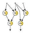
1/* ***************************** */ 2/* ******* feedback.cpp ***** */ 3 4/* 5 * ------------- 6 * | | 7 * | --> F -- 8 * v | . 9 * Stage0 --> Sched | . 10 * ˆ | . 11 * | --> F -- 12 * | | 13 * ------------- 14 */ 15#include <ff/farm.hpp> 16#include <ff/pipeline.hpp> 17using namespace ff; 18const long streamlength=20; 19 20long *F(long *in,ff_node*const) { 21 *in *= *in; 22 return in; 23} 24struct Sched: ff_node_t<long> { 25 Sched(ff_loadbalancer *const lb):lb(lb) {} 26 long* svc(long *task) { 27 int channel=lb->get_channel_id(); 28 if (channel == -1) { 29 std::cout << ”Task ” << *task << ” coming from Stage0\n”; 30 return task; 31 } 32 std::cout << ”Task ” << *task << ” coming from Worker” << channel << ”\n”; 33 delete task; 34 return GO_ON; 35 } 36 void eosnotify(ssize_t) { 37 // received EOS from Stage0, broadcast EOS to all workers 38 lb->broadcast_task(EOS); 39 } 40 ff_loadbalancer *lb; 41}; 42long *Stage0(long*, ff_node*const node) { 43 for(long i=0;i<streamlength;++i) 44 node->ff_send_out(new long(i)); 45 return (long*)EOS; 46} 47int main() { 48 ff_Farm<long> farm(F, 3); 49 farm.remove_collector(); // removes the default collector 50 // the scheduler gets in input the internal load-balancer 51 Sched S(farm.getlb()); 52 farm.add_emitter(S); 53 // adds feedback channels between each worker and the scheduler 54 farm.wrap_around(); 55 // creates a node from a function 56 ff_node_F<long> stage(Stage0); 57 // creates the pipeline 58 ff_Pipe<> pipe(stage, farm); 59 if (pipe.run_and_wait_end()<0) error(”running pipe”); 60 return 0; 61}
In this case the Emitter node of the farm receives tasks both from the first
stage of the pipeline and from farm’s workers. To discern different inputs
it is used the ff_get_channel_id method of the ff_loadbalancer
object: inputs coming from workers have channel id greater than 0 (the
channel id correspond to the worker id). The Emitter non-deterministic way
processes input tasks giving higher priority to the tasks coming back from
workers.
It is important to note how EOS propagation works in presence of loopback
channels. Normally, the EOS is automatically propagated onward by the FastFlow
run-time in order to implement pipeline-like termination. When internal loopback
channels are present in the skeleton tree (and in general when there is multi-input
nodes), the EOS is propagated only if the EOS message has been received from all
input channels. In this case is useful to be notified when an EOS is received so that
the termination can be controlled by the programmer. In the proposed example
above, we want to propagate the EOS as soon as we receive it from the Stage0 and
then to terminate the execution only after having received all EOS from all
workers.
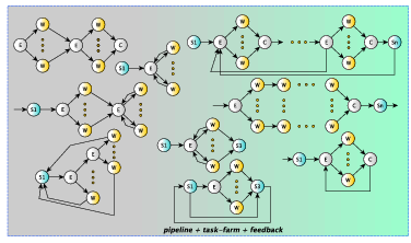
3.6 Mixing farms pipelines and feedbacks
FastFlow pipeline, task-farm skeletons and the feedback pattern modifier can be
nested and combined in many different ways. Figure 3.4 sketches some of the
possible combinations that can be realised in a easy way.
3.7 Software accelerators
FastFlow can be used to accelerate existing sequential code without the need of
completely restructuring the entire application using algorithmic skeletons. In a
nutshell, programmers may identify potentially concurrent tasks within the sequential
code and request their execution from an appropriate FastFlow pattern on the
fly.
By analogy with what happens with GPGPUs and FPGAs used to support
computations on the main processing unit, the cores used to run the user defined
tasks through FastFlow define a software ”accelerator” device. This device will run on
the ”spare” cores available. FastFlow accelerator is a ”software device” that can be
used to speedup portions of code using the cores left unused by the main application.
From a more formal perspective, a FastFlow accelerator is defined by a skeletal
composition augmented with an input and an output stream that can be,
respectively, pushed and popped from outside the accelerator. Both the functional
and extra-functional behaviour of the accelerator is fully determined by the chosen
skeletal composition.
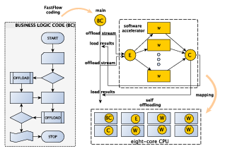
Using FastFlow accelerator mode is not that different from using FastFlow to write
an application only using skeletons (see Fig. 3.5). The skeletons must be
started as a software accelerator, and tasks have to be offloaded from the main
program. A simple program using the FastFlow accelerator mode is shown below:
1/* ***************************** */ 2/* ******* accelerator.cpp ***** */ 3 4#include <vector> 5#include <ff/farm.hpp> 6using namespace ff; 7struct Worker: ff_node_t<long> { 8 long *svc(long *task) { 9 *task = pow(*task,3); 10 return task; 11 } 12}; 13int main(int argc, char *argv[]) { 14 assert(argc>2); 15 int nworkers = atoi(argv[1]); 16 int streamlen= atoi(argv[2]); 17 18 std::vector<std::unique_ptr<ff_node> > Workers; 19 for(int i=0;i<nworkers;++i) 20 Workers.push_back(make_unique<Worker>()); 21 22 ff_Farm<long> farm(std::move(Workers), 23 true /* accelerator mode turned on*/); 24 // Now run the accelator asynchronusly 25 if (farm.run_then_freeze()<0) // farm.run() can also be used here 26 error(”running farm”); 27 long *result = nullptr; 28 for (long i=0;i<streamlen;i++) { 29 long *task = new long(i); 30 // Here offloading computation onto the farm 31 farm.offload(task); 32 33 // do something smart here... 34 for(volatile long k=0; k<10000; ++k); 35 36 // try to get results, if there are any 37 if (farm.load_result_nb(result)) { 38 std::cerr << ”[inside for loop] result= ” << *result << ”\n”; 39 delete result; 40 } 41 } 42 farm.offload(EOS); // sending End-Of-Stream 43#if 1 44 // get all remaining results syncronously. 45 while(farm.load_result(result)) { 46 std::cerr << ”[outside for loop] result= ” << *result << ”\n”; 47 delete result; 48 } 49#else 50 // asynchronously waiting for results 51 do { 52 if (farm.load_result_nb(result)) { 53 if (result==EOS) break; 54 std::cerr << ”[outside for loop] result= ” << *result << ”\n”; 55 delete result; 56 } 57 } while(1); 58#endif 59 farm.wait(); // wait for termination 60 return 0; 61}
The ”true” parameter in the farm constructor (the same is for the pipeline) is the
one telling the run-time that the farm (or pipeline) has to be used as an
accelerator. The idea is to start (or re-start) the accelerator and whenever we
have a task ready to be submitted to the accelerator, we simply ”offload” it
to the accelerator. When we have no more tasks to offload, we send the
End-Of-Stream and eventually we wait for the completion of the computation of
tasks in the accelerator or, we can wait_freezing to temporary stop the
accelerator without terminating the threads in order to restart the accelerator
afterwards.
The bool load_result(void ⋆⋆) methods synchronously await for one item
being delivered on the accelerator output stream. If such item is available, the
method returns ”true” and stores the item pointer in the parameter. If no other
items will be available, the method returns ”false”. An asynchronous method is also
available with signature bool load_results_nb(void ⋆⋆) When the method is
called, if no result is available, it returns ”false”, and might retry later on to see
whether a result is ready.
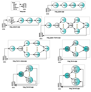
3.8 Examples
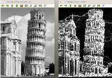
In this sections we consider an images filtering application in which 2 image filters
have to be applied to a stream of images. We prove different possible FastFlow
implementation using both pipeline and task-farm skeletons. The different
implementations described in the following are sketched in Fig. 3.6 (all but
versions img_farm2.cpp and img_farm3.cpp are reported as source code in this
tutorial): the starting sequential implementation (img.cpp), a 4-stage FastFlow
pipeline implementation (img_pipe.cpp), the same version as before but
the pipeline (3-stage) is implemented as a ”software accelerator” while the
image reader stage is directly the main program (img_pipe2.cpp), a 4-stage
FastFlow pipeline with the second and third stages implemented as task-farm
skeletons (img_pipe+farm.cpp), a variant of the previous case, i.e. a 3-stage
pipeline whose middle stage is a farm whose workers are 2-stage pipelines
(img_farm+pipe.cpp), and finally the so called ”normal-form”, i.e. a single task-farm
having the image reader stage collapsed with the farm Emitter and having
the image writer stage collapsed with the farm collector (img_farm.cpp).
The last 2 versions (not reported as source code here), i.e. img_farm2.cpp
and img_farm3.cpp, are incremental optimizations of the base img_farm.cpp
version in which the input and output is performed in parallel in the farm’s
workers.
3.8.1 Images filtering
Let’s consider a simple streaming application: two image filters (blur and emboss)
have to be applied to a stream of input images. The stream can be of any length and
images of any size (and of different format). For the sake of simplicity images’ file are
stored in a disk directory and the file names are passed as command line arguments
of our simple application. The output images are stored with the same name in a
separate directory.
The application uses the ImageMagick
library
to manipulate the images and to apply the two filters. In case the ImageMagick
library is not installed, please refer to the ”Install from Source” instructions
contained in the project web site. This is our starting sequential program:
1/* ********************* */ 2/* ******* img.cpp ***** */ 3 4#include <cassert> 5#include <iostream> 6#include <string> 7#include <algorithm> 8#include <Magick++.h> 9using namespace Magick; 10 11// helping functions: it parses the command line options 12char* getOption(char **begin, char **end, const std::string &option) { 13 char **itr = std::find(begin, end, option); 14 if (itr != end && ++itr != end) return *itr; 15 return nullptr; 16} 17int main(int argc, char *argv[]) { 18 double radius = 1.0; 19 double sigma = 0.5; 20 if (argc < 2) { 21 std::cerr << ”use: ” << argv[0] << ” [-r radius=1.0] [-s sigma=.5] image-files\n”; 22 return -1; 23 } 24 int start = 1; 25 char *r = getOption(argv, argv+argc, ”-r”); 26 char *s = getOption(argv, argv+argc, ”-s”); 27 if (r) { radius = atof(r); start+=2; argc-=2; } 28 if (s) { sigma = atof(s); start+=2; argc-=2; } 29 30 InitializeMagick(*argv); 31 32 long num_images = argc-1; 33 assert(num_images >= 1); 34 // for each image apply the 2 filter in sequence 35 for(long i=0; i<num_images; ++i) { 36 const std::string &filepath(argv[start+i]); 37 std::string filename; 38 39 // get only the filename 40 int n=filepath.find_last_of(”/”); 41 if (n>0) filename = filepath.substr(n+1); 42 else filename = filepath; 43 44 Image img; 45 img.read(filepath); 46 47 img.blur(radius, sigma); 48 img.emboss(radius, sigma); 49 50 std::string outfile = ”./out/” + filename; 51 img.write(outfile); 52 std::cout << ”image ” << filename 53 << ” has been written to disk\n”; 54 } 55 return 0; 56}
Since the two filters may be applied in sequence to independent input images, we
can compute the two filters in pipeline. So we define a 4-stage pipeline: the
first stage read images from the disk, the second and third stages apply the
two filters and the forth stage writes the resulting image into the disk (in a
separate directory). The code for implementing the pipeline is in the following:
1/* ************************** */ 2/* ******* img_pipe.cpp ***** */ 3 4/* 5 * Read --> Blur --> Emboss --> Write 6 * 7 */ 8#include <cassert> 9#include <iostream> 10#include <string> 11#include <algorithm> 12 13#include <ff/pipeline.hpp> 14#include <Magick++.h> 15using namespace Magick; 16using namespace ff; 17// this is the input/output task containing all information needed 18struct Task { 19 Task(Image *image, const std::string &name, double r=1.0,double s=0.5): 20 image(image),name(name),radius(r),sigma(s) {}; 21 22 Image *image; 23 const std::string name; 24 const double radius,sigma; 25}; 26 27char* getOption(char **begin, char **end, const std::string &option) { 28 char **itr = std::find(begin, end, option); 29 if (itr != end && ++itr != end) return *itr; 30 return nullptr; 31} 32// 1st stage 33struct Read: ff_node_t<Task> { 34 Read(char **images, const long num_images, double r, double s): 35 images((const char**)images),num_images(num_images),radius(r),sigma(s) {} 36 37 Task *svc(Task *) { 38 for(long i=0; i<num_images; ++i) { 39 const std::string &filepath(images[i]); 40 std::string filename; 41 42 // get only the filename 43 int n=filepath.find_last_of(”/”); 44 if (n>0) filename = filepath.substr(n+1); 45 else filename = filepath; 46 47 Image *img = new Image;; 48 img->read(filepath); 49 Task *t = new Task(img, filename,radius,sigma); 50 ff_send_out(t); // sends the task t to the next stage 51 } 52 return EOS; // computation completed 53 } 54 const char **images; 55 const long num_images; 56 const double radius,sigma; 57}; 58// function executed by the 2nd stage 59Task* BlurFilter(Task *in, ff_node*const) { 60 in->image->blur(in->radius, in->sigma); 61 return in; 62} 63// function executed by the 3rd stage 64Task* EmbossFilter(Task *in, ff_node*const) { 65 in->image->emboss(in->radius, in->sigma); 66 return in; 67} 68// function executed by the 4th stage 69Task* Write(Task* in, ff_node*const) { 70 std::string outfile = ”./out/” + in->name; 71 in->image->write(outfile); 72 std::cout << ”image ” << in->name << ” has been written to disk\n”; 73 delete in->image; 74 delete in; 75 return (Task*)GO_ON; 76} 77 78int main(int argc, char *argv[]) { 79 if (argc < 2) { 80 std::cerr << ”use: ” << argv[0] 81 << ” [-r radius=1.0] [-s sigma=.5] image-files\n”; 82 return -1; 83 } 84 double radius=1.0,sigma=0.5; 85 int start = 1; 86 char *r = getOption(argv, argv+argc, ”-r”); 87 char *s = getOption(argv, argv+argc, ”-s”); 88 if (r) { radius = atof(r); start+=2; argc-=2; } 89 if (s) { sigma = atof(s); start+=2; argc-=2; } 90 91 InitializeMagick(*argv); 92 long num_images = argc-1; 93 assert(num_images >= 1); 94 95 Read read(&argv[start], num_images, radius, sigma); // 1st stage 96 ff_node_F<Task> blur(BlurFilter); // 2nd stage 97 ff_node_F<Task> emboss(EmbossFilter); // 3nd stage 98 ff_node_F<Task> write(Write); // 4th stage 99 ff_Pipe<> pipe(read,blur,emboss,write); 100 101 if (pipe.run_and_wait_end()<0) { // executes the pipeline 102 error(”running pipeline\n”); 103 return -1; 104 } 105 return 0; 106}
It is possible to instantiate the pipeline as a software accelerator. In the following
we report only the code of the main function since it is the only part of the code that
differs:
1/* *************************** */ 2/* ******* img_pipe2.cpp ***** */ 3 4/* 5 * main 6 * | 7 * ->| 8 * | Read 9 * | offload ---> pipeline( BlurFilter, EmbossFilter, Write ) 10 * - | 11 * | 12 */ 13int main(int argc, char *argv[]) { 14 if (argc < 2) { 15 std::cerr << ”use: ” << argv[0] 16 << ” [-r radius=1.0] [-s sigma=.5] image-files\n”; 17 return -1; 18 } 19 double radius=1.0,sigma=0.5; 20 int start = 1; 21 char *r = getOption(argv, argv+argc, ”-r”); 22 char *s = getOption(argv, argv+argc, ”-s”); 23 if (r) { radius = atof(r); start+=2; argc-=2; } 24 if (s) { sigma = atof(s); start+=2; argc-=2; } 25 26 InitializeMagick(*argv); 27 28 long num_images = argc-1; 29 assert(num_images >= 1); 30 31 ff_node_F<Task> blur(BlurFilter); 32 ff_node_F<Task> emboss(EmbossFilter); 33 ff_node_F<Task> write(Write); 34 35 ff_Pipe<> pipe(true, // enable accelerator 36 blur, // 2nd stage 37 emboss, // 3rd stage 38 write); // 4th stage 39 40 if (pipe.run_then_freeze()<0) { // start the pipeline 41 error(”running pipeline\n”); 42 return -1; 43 } 44 for(long i=0; i<num_images; ++i) { 45 const std::string &filepath(argv[start+i]); 46 std::string filename; 47 48 // get only the filename 49 int n=filepath.find_last_of(”/”); 50 if (n>0) filename = filepath.substr(n+1); 51 else filename = filepath; 52 53 Image *img = new Image;; 54 img->read(filepath); 55 Task *t = new Task(img, filename,radius,sigma); 56 pipe.offload(t); // sends the task t to the pipeline 57 } 58 pipe.offload(EOS); // sends the End-Of-Stream 59 60 if (pipe.wait()<0) { // wait for pipeline termination 61 error(”waiting pipeline\n”); 62 return -1; 63 } 64 return 0; 65}
Now, since the same filter may be applied in parallel to independent input images,
we can replace the second and third stage with two task-farm having the same
previous stage as worker. This is safe because we know that we can replicate the
function computing the filters: it is thread safe and has no internal shared state. The
resulting code is:
1/* ******************************* */ 2/* ******* img_pipe+farm.cpp ***** */ 3 4/* 5 * --> Blur -- --> Emboss -- 6 * | | | | 7 * Read --> Sched |--> Blur --|-- >Sched |--> Emboss --| --> Write 8 * | | | | 9 * --> Blur -- --> Emboss -- 10 */ 11#include <cassert> 12#include <iostream> 13#include <string> 14#include <algorithm> 15#include <ff/pipeline.hpp> 16#include <ff/farm.hpp> 17#include <Magick++.h> 18using namespace Magick; 19using namespace ff; 20struct Task { 21 Task(Image *image, const std::string &name, double r=1.0,double s=0.5): 22 image(image),name(name),radius(r),sigma(s) {}; 23 Image *image; 24 const std::string name; 25 const double radius,sigma; 26}; 27typedef std::function<Task*(Task*,ff_node*const)> fffarm_f; 28char* getOption(char **begin, char **end, const std::string &option) { 29 char **itr = std::find(begin, end, option); 30 if (itr != end && ++itr != end) return *itr; 31 return nullptr; 32} 33// 1st stage 34struct Read: ff_node_t<Task> { 35 Read(char **images, const long num_images, double r, double s): 36 images((const char**)images),num_images(num_images),radius(r),sigma(s) {} 37 38 Task *svc(Task *) { 39 for(long i=0; i<num_images; ++i) { 40 const std::string &filepath(images[i]); 41 std::string filename; 42 43 // get only the filename 44 int n=filepath.find_last_of(”/”); 45 if (n>0) filename = filepath.substr(n+1); 46 else filename = filepath; 47 48 Image *img = new Image;; 49 img->read(filepath); 50 Task *t = new Task(img, filename,radius,sigma); 51 std::cout << ”sending out ” << filename << ”\n”; 52 ff_send_out(t); // sends the task t to the next stage 53 } 54 return EOS; // computation completed 55 } 56 const char **images; 57 const long num_images; 58 const double radius, sigma; 59}; 60// function executed by the 2nd stage 61Task* BlurFilter(Task *in, ff_node*const) { 62 in->image->blur(in->radius, in->sigma); 63 return in; 64} 65// function executed by the 3rd stage 66Task* EmbossFilter(Task *in, ff_node*const) { 67 in->image->emboss(in->radius, in->sigma); 68 return in; 69} 70// function executed by the 4th stage 71Task *Write(Task* in, ff_node*const) { 72 std::string outfile = ”./out/” + in->name; 73 in->image->write(outfile); 74 std::cout << ”image ” << in->name << ” has been written to disk\n”; 75 delete in->image; 76 delete in; 77 return (Task*)GO_ON; 78} 79// 4th stage 80struct Writer: ff_minode_t<Task> { // this is a multi-input node 81 Task *svc(Task *task) { 82 return Write(task, this); 83 } 84}; 85 86int main(int argc, char *argv[]) { 87 if (argc < 2) { 88 std::cerr << ”use: ” << argv[0] 89 << ” [-r radius=1.0]” 90 << ” [-s sigma=.5]” 91 << ” [ -n blurWrk=2]” 92 << ” [ -m embossWrk=2] image-files\n”; 93 return -1; 94 } 95 double radius=1.0,sigma=0.5; 96 int blurWrk = 2, embossWrk = 2; 97 int start = 1; 98 char *r = getOption(argv, argv+argc, ”-r”); 99 char *s = getOption(argv, argv+argc, ”-s”); 100 char *n = getOption(argv, argv+argc, ”-n”); 101 char *m = getOption(argv, argv+argc, ”-m”); 102 if (r) { radius = atof(r); start+=2; argc-=2; } 103 if (s) { sigma = atof(s); start+=2; argc-=2; } 104 if (n) { blurWrk = atoi(n); start+=2; argc-=2; } 105 if (m) { embossWrk = atoi(m); start+=2; argc-=2; } 106 107 InitializeMagick(*argv); 108 109 long num_images = argc-1; 110 assert(num_images >= 1); 111 112 ff_Farm<Task> blurFarm(BlurFilter,blurWrk); 113 blurFarm.remove_collector(); 114 blurFarm.set_scheduling_ondemand(); 115 ff_Farm<Task> embossFarm(EmbossFilter,embossWrk); 116 // this is needed because the previous farm does not has the Collector 117 embossFarm.setMultiInput(); 118 embossFarm.remove_collector(); 119 embossFarm.set_scheduling_ondemand(); 120 Read read(&argv[start], num_images, radius, sigma); 121 Writer write; 122 ff_Pipe<> pipe(read, // 1st stage 123 blurFarm, // 2nd stage 124 embossFarm, // 3rd stage 125 write); // 4th stage 126 if (pipe.run_and_wait_end()<0) { // executes the pipeline 127 error(”running pipeline\n”); 128 return -1; 129 } 130 return 0; 131}
A possible variant of the previous implementation, which uses only one scheduler
is the following one:
1/* ******************************* */ 2/* ******* img_farm+pipe.cpp ***** */ 3 4/* 5 * --> Blur --> Emboss -- 6 * | | 7 * Read --> Sched -|--> Blur --> Emboss --| -->Write 8 * | | 9 * --> Blur --> Emboss -- 10 * 11 */ 12#include <cassert> 13#include <iostream> 14#include <string> 15#include <algorithm> 16 17#include <ff/pipeline.hpp> 18#include <ff/farm.hpp> 19#include <Magick++.h> 20using namespace Magick; 21using namespace ff; 22struct Task { 23 Task(Image *image, const std::string &name, double r=1.0,double s=0.5): 24 image(image),name(name),radius(r),sigma(s) {}; 25 26 Image *image; 27 const std::string name; 28 const double radius; 29 const double sigma; 30}; 31char* getOption(char **begin, char **end, const std::string &option) { 32 char **itr = std::find(begin, end, option); 33 if (itr != end && ++itr != end) return *itr; 34 return nullptr; 35} 36// 1st stage 37struct Read: ff_node_t<Task> { 38 Read(char **images, const long num_images, double r, double s): 39 images((const char**)images),num_images(num_images),radius(r),sigma(s) {} 40 41 Task *svc(Task *) { 42 for(long i=0; i<num_images; ++i) { 43 const std::string &filepath(images[i]); 44 std::string filename; 45 46 // get only the filename 47 int n=filepath.find_last_of(”/”); 48 if (n>0) filename = filepath.substr(n+1); 49 else filename = filepath; 50 51 Image *img = new Image;; 52 img->read(filepath); 53 Task *t = new Task(img, filename,radius,sigma); 54 std::cout << ”sending out ” << filename << ”\n”; 55 ff_send_out(t); // sends the task t to the next stage 56 } 57 return EOS; // computation completed 58 } 59 60 const char **images; 61 const long num_images; 62 const double radius, sigma; 63}; 64// function executed by the 2nd stage 65Task* BlurFilter(Task *in, ff_node*const) { 66 in->image->blur(in->radius, in->sigma); 67 return in; 68 69} 70// function executed by the 3rd stage 71Task* EmbossFilter(Task *in, ff_node*const) { 72 in->image->emboss(in->radius, in->sigma); 73 return in; 74} 75// function executed by the 4th stage 76Task *Write(Task* in, ff_node*const) { 77 std::string outfile = ”./out/” + in->name; 78 in->image->write(outfile); 79 std::cout << ”image ” << in->name << ” has been written to disk\n”; 80 delete in->image; 81 delete in; 82 return (Task*)GO_ON; 83} 84// 4th stage 85struct Writer: ff_minode_t<Task> { // this is a multi-input node 86 Task *svc(Task *task) { 87 return Write(task, this); 88 } 89}; 90 91int main(int argc, char *argv[]) { 92 if (argc < 2) { 93 std::cerr << ”use: ” << argv[0] 94 << ” [-r radius=1.0]” 95 << ” [-s sigma=.5]” 96 << ” [ -n Wrk=2] image-files\n”; 97 return -1; 98 } 99 double radius=1.0,sigma=0.5; 100 int Wrks = 2; 101 int start = 1; 102 char *r = getOption(argv, argv+argc, ”-r”); 103 char *s = getOption(argv, argv+argc, ”-s”); 104 char *n = getOption(argv, argv+argc, ”-n”); 105 if (r) { radius = atof(r); start+=2; argc-=2; } 106 if (s) { sigma = atof(s); start+=2; argc-=2; } 107 if (n) { Wrks = atoi(n); start+=2; argc-=2; } 108 109 InitializeMagick(*argv); 110 111 long num_images = argc-1; 112 assert(num_images >= 1); 113 114 std::vector<std::unique_ptr<ff_node> > W; 115 for(int i=0;i<Wrks;++i) 116 W.push_back(make_unique<ff_Pipe<Task> >(make_unique<ff_node_F<Task> >(BlurFilter), 117 make_unique<ff_node_F<Task> >(EmbossFilter))); 118 ff_Farm<Task> farm(std::move(W)); 119 farm.remove_collector(); 120 farm.set_scheduling_ondemand(); // set auto scheduling 121 122 Read read(&argv[start], num_images, radius, sigma); 123 Writer write; 124 ff_Pipe<> pipe(read, // 1st stage 125 farm, // 2nd stage 126 write); // 3th stage 127 if (pipe.run_and_wait_end()<0) { // executes the pipeline 128 error(”running pipeline\n”); 129 return -1; 130 } 131 return 0; 132}
The next step is to reduce the number of resources used. For example the farm
Emitter can be used to read files from the disk, whereas the farm Collector for
writing files to the disk. Furthermore, the blur and emboss filters may be computed
sequentially using a single workers. This is the so called ”normal form” obtained
optimising the resource usage. The code implementing the normal form is the
following:
1/* ************************** */ 2/* ******* img_farm.cpp ***** */ 3 4/* 5 * 6 * --> Blur+Emboss -- 7 * | | 8 * Read+Sched --|--> Blur+Emboss --|-->Collector+Write 9 * | | 10 * --> Blur+Emboss -- 11 */ 12#include <cassert> 13#include <iostream> 14#include <string> 15#include <algorithm> 16 17#define HAS_CXX11_VARIADIC_TEMPLATES 1 18#include <ff/pipeline.hpp> 19#include <ff/farm.hpp> 20#include <Magick++.h> 21using namespace Magick; 22using namespace ff; 23struct Task { 24 Task(Image *image, const std::string &name, double r=1.0,double s=0.5): 25 image(image),name(name),radius(r),sigma(s) {}; 26 27 Image *image; 28 const std::string name; 29 const double radius, sigma; 30}; 31char* getOption(char **begin, char **end, const std::string &option) { 32 char **itr = std::find(begin, end, option); 33 if (itr != end && ++itr != end) return *itr; 34 return nullptr; 35} 36// 1st stage 37struct Read: ff_node_t<Task> { 38 Read(char **images, const long num_images, double r, double s): 39 images((const char**)images),num_images(num_images),radius(r),sigma(s) {} 40 41 Task *svc(Task *) { 42 for(long i=0; i<num_images; ++i) { 43 const std::string &filepath(images[i]); 44 std::string filename; 45 46 // get only the filename 47 int n=filepath.find_last_of(”/”); 48 if (n>0) filename = filepath.substr(n+1); 49 else filename = filepath; 50 51 Image *img = new Image;; 52 img->read(filepath); 53 Task *t = new Task(img, filename,radius,sigma); 54 std::cout << ”sending out ” << filename << ”\n”; 55 ff_send_out(t); // sends the task t to the next stage 56 } 57 return EOS; // computation completed 58 } 59 60 const char **images; 61 const long num_images; 62 const double radius,sigma; 63}; 64// function executed by the 2nd stage 65Task* BlurFilter(Task *in, ff_node*const) { 66 in->image->blur(in->radius, in->sigma); 67 return in; 68 69} 70// function executed by the 3rd stage 71Task* EmbossFilter(Task *in, ff_node*const) { 72 in->image->emboss(in->radius, in->sigma); 73 return in; 74} 75struct BlurEmbossWrapper: ff_node_t<Task> { 76 Task *svc(Task *task) { 77 return EmbossFilter(BlurFilter(task,this),this); 78 } 79}; 80 81// function executed by the 4th stage 82Task *Write(Task* in, ff_node*const) { 83 std::string outfile = ”./out/” + in->name; 84 in->image->write(outfile); 85 std::cout << ”image ” << in->name << ” has been written to disk\n”; 86 delete in->image; 87 delete in; 88 return (Task*)GO_ON; 89} 90// 4th stage 91struct Writer: ff_minode_t<Task> { // this is a multi-input node 92 Task *svc(Task *task) { 93 return Write(task, this); 94 } 95}; 96 97int main(int argc, char *argv[]) { 98 if (argc < 2) { 99 std::cerr << ”use: ” << argv[0] 100 << ” [-r radius=1.0]” 101 << ” [-s sigma=.5]” 102 << ” [ -n Wrks=2]” 103 << ” [ -m Wrk=2] image-files\n”; 104 return -1; 105 } 106 double radius=1.0,sigma=0.5; 107 int Wrks = 2; 108 int start = 1; 109 char *r = getOption(argv, argv+argc, ”-r”); 110 char *s = getOption(argv, argv+argc, ”-s”); 111 char *n = getOption(argv, argv+argc, ”-n”); 112 if (r) { radius = atof(r); start+=2; argc-=2; } 113 if (s) { sigma = atof(s); start+=2; argc-=2; } 114 if (n) { Wrks = atoi(n); start+=2; argc-=2; } 115 116 InitializeMagick(*argv); 117 long num_images = argc-1; 118 assert(num_images >= 1); 119 120 std::vector<std::unique_ptr<ff_node> > W; 121 for(int i=0;i<Wrks;++i) 122 W.push_back(make_unique<BlurEmbossWrapper>()); 123 124 Read read(&argv[start], num_images, radius, sigma); 125 Writer writer; 126 ff_Farm<Task> farm(std::move(W), read, writer); 127 farm.set_scheduling_ondemand(); 128 129 if (farm.run_and_wait_end()<0) { // executes the task-farm 130 error(”running pipeline\n”); 131 return -1; 132 } 133 return 0; 134}
Chapter 4
Data parallelism
In data parallel computation, data structures (typically large) are partitioned among
the number of concurrent resources each of which computes the same function on the
assigned partition. In a nutshell, the input task, possibly but not necessarily coming
from an input stream, is split into multiple sub-task each one computed in parallel
and then collected together in one single output task. The computation on the
sub-tasks may be completely independent (i.e. the sub-task computation uses data
only coming from the the current sub-task) or dependent on previously computed
data (non necessarily in the corresponding sub-task). The main goal of data parallel
computation is to reduce the completion time of the single task to compute. It is
important to note that, data decomposition using large sub-tasks, together
with static assignment of such partitions to workers, may introduce load
imbalance during the computation mainly because of the variable calculation
time associated to distinct partitions. In general, it is possible to state that
load balancing is a feature of anonymous task assignment, i.e. tasks to be
computed are dynamically assigned to available computing resources, without
a-priori correspondence between tasks and available computing resources.
The task-farm paradigm is naturally based on this concept (where tasks are
stream items), and for this reason quite often data-parallel computations are
implemented on top of the task-farm skeleton by using the auto-scheduling
policy (see Sec. 3.3). Many other scheduling strategies have been devised for
balancing data-parallel computations, among these, the work-stealing scheduling
strategy is of particular importance. It is worth to note here that, when the
task-farm is used to implement an unbalanced data parallel computation, it is
possible to ”customise” it to use a work-stealing scheduling strategy. In other
words, the task-farm pattern just models functional replication, while data
partitioning and task-scheduling depends on the way the Emitter entity is
implemented.
Well known and widely used data parallel skeletons are: map reduce and
stencil.
4.1 Data parallel skeletons
In this section we describe map-like and reduce-like patterns, whereas the stencil
pattern is not covered.
map
The simplest data parallel computation is the map, in which the concurrent workers
operating on a partition of the input data structure (typically an N-dimensional
array) are fully independent, i.e. each of them operates on its own local data only,
without any cooperation with other computing resources. As an example consider the
following piece of code:
1const size_t N = 1<<15; 2long A[N],B[N]; 3for(size_t i=1; i<N; ++i) 4 A[i-1] = F(B[i]); 5A[N-1] = F(B[0]);
If the function F has no internal state, each loop iteration may be computed
independently since there are no true dependency among iterations. In this case we
may apply the map pattern, splitting the two arrays A,B in n =  parts and
assign each part to one worker. Each worker executes the same loop as above on a
restricted index range. In principle, the execution time can be reduced by a factor of
n if we consider a run-time with zero overhead, and as a particular case, if
nworkers = N, the execution time is reduced from O(N) to O(1). It is worth to note
that, the map skeleton may be simply implemented using a task-farm skeleton
operating on a single input data. The Emitter split the input arrays and distributes
the partitions to each worker. The workers apply the function F on the input
partition, finally the Collector collects the workers’ partitions in one single output
task.
parts and
assign each part to one worker. Each worker executes the same loop as above on a
restricted index range. In principle, the execution time can be reduced by a factor of
n if we consider a run-time with zero overhead, and as a particular case, if
nworkers = N, the execution time is reduced from O(N) to O(1). It is worth to note
that, the map skeleton may be simply implemented using a task-farm skeleton
operating on a single input data. The Emitter split the input arrays and distributes
the partitions to each worker. The workers apply the function F on the input
partition, finally the Collector collects the workers’ partitions in one single output
task.
Loop-parallelism
A sequential iterative kernel with independent iterations is also known as a parallel
loop. Parallel loops may be clearly parallelized by using the map or farm skeletons,
but this typically requires a substantial re-factoring of the original loop code with the
possibility to introduce bugs and not preserving sequential equivalence. Furthermore,
the selection of the appropriate implementation skeleton together with a correct
implementation of the sequential wrapper code is of foremost importance for
obtaining the best performance.
For these reasons, in the FastFlow framework there are a set of data parallel
patterns implemented on top of the basic FastFlow skeletons to ease the
implementation of parallel loops.
4.2 FastFlow abstractions
In this section we describe the different parallel-for abstractions that are used to
implement almost all data-parallel skeletons currently available in the FastFlow
framework for multi-core systems.
4.2.1 ParallelFor
Here we introduce the FastFlow ParallelFor pattern that can be used to parallelize
loops having independent iterations:
for(long idx=first; idx < last; idx += step) bodyF;
The class interface of the ParallelFor pattern is described in the parallel_for.hpp
file. The constructor accepts two parameters:
ParallelFor(const long maxnworkers=FF_AUTO,bool spinWait=false);
the first parameter sets the maximum number of worker threads that can be used in
the ParallelFor (that is the maximum concurrency degree), the second argument sets
non-blocking run-time for parallel computations. At the beginning you may just leave
the default parameters for these two arguments.
The ParallelFor object, encapsulates a number of parallel_for
methods, which differentiate each other for the number of arguments they
get and for the signatures of the function body. A single ParallelFor object
can be used as many times as needed to run different parallel-for instances
(different loop bodies). Nested invocations of ParallelFor methods are not
supported.
The loop body may be a standard function or a C++11 lambda-function. A
C++11 lambda-function is a new feature of the C++11 standard already supported
by many compilers. They are unnamed closures (i.e. function objects that can be
constructed and managed like data) that allow functions to be syntactically defined
where and when needed. When lambda functions are built, they can capture the
state of non-local variables named in the wrapped code either by value or by
reference.
The following list presents the most useful parallel-for methods provided by the
ParallelFor class:
parallel_for(first,last, bodyF, nworkers);// step=1,grain=FF_AUTO
parallel_for(first,last,step, bodyF, nworkers);// grain=FF_AUTO
parallel_for(first,last,step,grain, bodyF, nworekrs);
bodyF = F(const long idx);
parallel_for_thid(first,last,step,grain, bodyF, nworkers);
bodyF = F(const long idx,const int thid);
// thid is the id of the thread executing the body function
parallel_for_idx(first,last,step,grain, bodyF, nworkers);
bodyF = F(const long begin,const long end,const int thid);
Now, given the following sequential loop:
auto F = [](const long i) { return i⋆i;}
for(long i=1; i < 100; i +=2) A[i] = F(i);
we can write the following parallel-for:
ParallelFor pf;
auto F = [](const long i) { return i⋆i;}
pf.parallel_for(1,100,2,[&A](const long i) { A[i]=F(i);});
or by using the parallel_for_idx we have:
ParallelFor pf;
auto F = [](const long i) { return i⋆i;}
pf.parallel_for_idx(1,100,2,[&A](const long begin,const long end,
const int thid){
std::cout << "Hello I'm thread " << thid
<< " executing iterations (" << start <<"," << end <<")\n";
for(long i=begin; i<end; i += 2) A[i]=F(i);
});
the parallel_for_idx is just a ”low-level” version of the parallel_for,
where the internal loop, iterating over all iterations assigned to the worker, has to be
written directly by the user. This may be useful when it is needed to execute a
pre-computation (executed in parallel) before starting the execution of the loop
iterations, or in general for debugging purposes.
It is important to remark that, when spinWait is set to true (see Sec. 4.2.1 for
details), in some particular cases, the body function is called the first time with
begin==end==0 so it would be safe to test this condition at the beginning of the
parallel_for_idx (i.e. if (begin==end) return;).
Let’s now see a very simple usage example of the parallel-for:
1/* ************************* */ 2/* ******* parfor1.cpp ***** */ 3 4#include <ff/parallel_for.hpp> 5using namespace ff; 6 7int main(int argc, char *argv[]) { 8 assert(argc>1); 9 long N = atol(argv[1]); 10 long *A = new long[N]; 11 ParallelFor pf; 12 // initialize the array A 13 pf.parallel_for(0,N,[&A](const long i) { A[i]=i;}); 14 // do something on each even element of the array A 15 pf.parallel_for(0,N,2,[&A](const long i) { A[i]=i*i;}); 16 // print the result 17 for(long i=0;i<N;++i) std::cout << A[i] << ” ”; 18 std::cout << ”\n”; 19 return 0; 20}
in this case, first the array A has been initialised using a parallel-for and
then the square value of the even entries is computed in parallel over N∕2
iterations.
Iterations scheduling
Three distinct iteration schedulings are currently possible in parallel-for
computations:
-
1.
- default static scheduling: the iteration space is (almost) evenly
partitioned in large contiguous chunks, and then they are statically
assigned to workers, one chunk for each worker.
-
2.
- static scheduling with interleaving k: the iteration space is statically
divided among all active workers in a round-robin fashion using a stride
of k. For example, to execute 10 iterations (from 0 to 9) using a
concurrency degree of 2 and a stride k = 3, then the first thread
executes iterations 0,1,2,6,7,8 and the second thread executes iterations
3,4,5,9. The default static scheduling is obtained setting a stride k =
iterationspace∕nworkers.
-
3.
- dynamic scheduling with chunk k: in this case no more than k
contiguous iterations at a time are dynamically assigned to computing
workers. As soon as a worker completes computation of one chunk of
iterations, a new chunk (if available) is selected and assigned to the worker.
The run-time tries to select as many as possible contiguous chunks in
order to better exploit spatial locality. This allows to have a good trade-off
between iterations affinity and load-balancing.
By default the default static scheduling is used. In general, the scheduling
policy is selected by specifying the grain parameter of the parallel_for
method. If the grain parameter is not specified or if its value is 0, then the
default static scheduling is selected. If grain is greater than zero, then the
dynamic scheduling is selected with k = grain. Finally, to use the static
scheduling with interleaving k the parallel_for_static method must be
used with k = grain. Note that, if in the parallel_for_static the
grain parameter is zero, than the default static scheduling policy is selected.
Summarising, in the following different scheduling strategies are selected
according to the grain parameter:
pf.parallel_for(1,100,2, bodyF); // default static sched.
pf.parallel_for(1,100,2, 0,bodyF); // default static sched.
pf.parallel_for(1,100,2,10,bodyF); // dynamic sched. with k=10
pf.parallel_for_static(1,100,2,10,bodyF);// static sched.
// interleaving k=10
pf.parallel_for_static(1,100,2,0,bodyF); // default static sched.
threadPause and disableScheduler
The spinWait parameter in the ParallelFor constructor enables non-blocking
computation between successive calls of parallel_for methods. This means that if
the parallel-for is not destructed and not used for a while, the worker threads will be
active in a busy waiting loop. In this case it may be useful to ”pause” the threads
until the parallel-for pattern is used again. To attain this, the threadPause method
can be used. The next time the parallel-for is used, the non-blocking run-time will be
still active.
Another interesting option of the ParallelFor object, is the possibility to
switch between two distinct run-time support for the scheduling of loop
iterations:
-
1.
- active scheduling where an active non-blocking scheduler thread (the
farm’s Emitter) is used to implement the auto-scheduling policy;
-
2.
- passive scheduling where workers cooperatively schedule tasks via
non-blocking synchronisations in memory.
Which one is better ? It is difficult to say, as it depends on many factors:
parallelism degree, task granularity and underlying platform, among others. As a rule
of thumb, on large multi-core and with fine-grain tasks active scheduling typically
runs faster; on the other hand, when there are more threads than available cores
the passive scheduler allows reduction of CPU conflicts obtaining better
performance.
By default, if the number of active workers is less than the number of available
cores, than the active scheduling is used. To dynamically switch between active
(false) and passive (true) scheduling strategies the disableScheduler method can
be used.
4.2.2 ParallelForReduce
The FastFlow ParallelForReduce is used to perform a parallel-for computation
plus a reduction operation (by using a combiner function named reduceF in the
following) over a sequence of elements of type T. In order to deterministically
compute the result, the reduction function needs to be associative and commutative.
The constructor interface is:
ParallelForReduce<T>(const long max=FF_AUTO,bool spinwait=false);
where the template type T is the type of the reduction variable, the first
parameter sets the maximum number of worker threads that can be used in the
ParallelForReduce, the second argument sets non-blocking run-time.
The ParallelForReduce class provides all the parallel-for methods already
provided by the ParallelFor class and a set of additional parallel_reduce
methods:
parallel_reduce(var,identity, first,last,
bodyF, reduceF, nworkers);// step=1,grain=FF_AUTO
parallel_reduce(var,identity, first,last,step,
bodyF, reduceF, nworkers);// grain=FF_AUTO
parallel_reduce(var,identity, first,last,step,grain,
bodyF, reduceF, nworekrs);
bodyF =F(const long idx,T& var);
reduceF =R(T& var,const T& elem);
parallel_reduce_thid(var,identity, first,last,step,grain,
bodyF, reduceF, nworkers);
bodyF =F(const long idx,T& var,const int thid);
reduceF =R(T& var,const T& elem);
// thid is the id of the thread executing the body function
parallel_reduce_idx(var,identity, first,last,step,grain,
bodyF, reduceF, nworkers);
bodyF =F(T& var,const long begin,const long end,const int thid);
reduceF =R(T& var,const T& elem);
The reduceF function specified in all parallel_reduce methods, executes the
reduction operation.
As an example, let’s consider the simple case of the sum of array’s elements:
1/* ************************** */ 2/* ******* arraysum.cpp ***** */ 3 4#include <iostream> 5#include <ff/parallel_for.hpp> 6using namespace ff; 7const size_t SIZE= 1<<20; 8int main(int argc, char * argv[]) { 9 assert(argc > 1); 10 int nworkers = atoi(argv[1]); 11 // creates the array 12 double *A = new double[SIZE]; 13 14 ParallelForReduce<double> pfr(nworkers); 15 // fill out the array A using the parallel-for 16 pfr.parallel_for(0,SIZE,1, 0, [&](const long j) { A[j]=j*1.0;}); 17 18 auto reduceF = [](double& sum, const double elem) { sum += elem; }; 19 auto bodyF = [&A](const long j, double& sum) { sum += A[j]; }; 20 { 21 double sum = 0.0; 22 std::cout << ”\nComputing sum with ” << std::max(1,nworkers/2) 23 << ” workers, default static scheduling\n”; 24 pfr.parallel_reduce(sum, 0.0, 0L, SIZE, 25 bodyF, reduceF, std::max(1,nworkers/2)); 26 std::cout << ”Sum = ” << sum << ”\n\n”; 27 } 28 { 29 double sum = 0.0; 30 std::cout << ”Computing sum with ” << nworkers 31 << ” workers, static scheduling with interleaving 1000\n”; 32 pfr.parallel_reduce_static(sum, 0.0, 0, SIZE, 1, 1000, 33 bodyF, reduceF, nworkers); 34 std::cout << ”Sum = ” << sum << ”\n\n”; 35 } 36 { 37 double sum = 0.0; 38 std::cout << ”Computing sum with ” << nworkers-1 39 << ” workers, dynamic scheduling chunk=1000\n”; 40 pfr.parallel_reduce(sum, 0.0, 0, SIZE, 1, 1000, 41 bodyF, reduceF, nworkers); 42 std::cout << ”Sum = ” << sum << ”\n\n”; 43 } 44 delete [] A; 45 return 0; 46}
in this simple test, we used a parallel-for for initialising the array A, and 3
parallel_reduce calls for computing the final sum (the reduction variable) using
the default static scheduling, the static scheduling with interleaving and the dynamic
scheduling, respectively.
4.2.3 ParallelForPipeReduce
The ParallelForPipeReduce uses a different skeleton implementation
of the ParallelForReduce pattern. The ParallelForPipeReduce
computes a map function and a sequential reduce function in a pipeline
fashion.
This pattern is useful in cases in which the reduce function has to be
computed sequentially, for example because there are concurrent write accesses in
some memory locations (so they have to be serialised using a lock). In these
cases, the typical solution is to execute the map part (for example using a
parallel-for) and then when the map is completed, execute the reduce part
sequentially and this may be expensive because a full barrier (between the
map and the reduce) is required. The ParallelForPipeReduce pattern
allows execution of the map and reduce part in pipeline without any barriers.
The ParallelForPipeReduce pattern is more complex to use than the
ParallelForReduce pattern because it requires to explicitly send the tasks to the
reduce stage inside the body of the map function. The ParallelForPipeReduce
class defined in the parallel_for.hpp file provides only 2 parallel-for
methods:
parallel_for_idx(first,last,step,grain,
mapF, nworkers);
mapF =F(const long begin,const long end,const int thid,
ff_buffernode& node);
parallel_reduce_idx(first,last,step,grain,
mapF, reduceF, nworkers);
mapF =F(const long begin,const long end,const int thid,
ff_buffernode& node);
reduceF =R(T& var);
As an example, let’s consider the same simple case implemented in the previous
section, i.e. the computation of the sum of array’s elements:
1/* *************************** */ 2/* ******* arraysum2.cpp ***** */ 3 4#include <ff/parallel_for.hpp> 5using namespace ff; 6const size_t SIZE= 1<<20; 7int main(int argc, char * argv[]) { 8 assert(argc > 1); 9 int nworkers = atoi(argv[1]); 10 // creates the array 11 double *A = new double[SIZE]; 12 ParallelForPipeReduce<double*> pfpipe(nworkers,true); 13 // init 14 pfpipe.parallel_for_idx(0,SIZE,1,0, 15 [&A](const long start,const long stop, 16 const int thid,ff_buffernode &) { 17 for(long j=start;j<stop;++j) A[j] = j*1.0; 18 }); 19 double sum = 0.0; 20 auto mapF = [&A](const long start,const long stop, 21 const int thid,ff_buffernode &node) { 22 // needed to avoid sending spurious lsum values to the reduce stage 23 if (start==stop) return; 24 double *lsum=new double(0.0); // allocate a task to send 25 for(long i=start;i<stop;++i) *lsum += A[i]; 26 node.put(lsum); // sending the partial sum to the next reduce stage 27 }; 28 auto reduceF = [&sum](double *lsum) { sum += *lsum; delete lsum; }; 29 std::cout << ”Computing sum with ” << nworkers 30 << ” workers, using the ParallelForPipeReduce and default sched.\n”; 31 pfpipe.parallel_reduce_idx(0, SIZE, 1, 0, mapF, reduceF); 32 std::cout << ”Sum = ” << sum << ”\n\n”; 33 delete [] A; 34 return 0; 35}
4.2.4 ff_Map
The FastFlow map parallel pattern is implemented as an ff_node_t abstraction and
a ParallelForReduce pattern. The idea is that, the map pattern is just an
interface to a parallel-for on multi-core platforms, while it provides a simple
abstraction for targeting multi-GPGPUs (both OpenCL and CUDA) and, in the
future versions, FPGAs on many-core platforms. The ff_Map<S,T> is a template
class accepting three template parameters: the first two are the type of the
input-output task (i.e. the template parameter of the ff_node_t<IN,OUT>
class); the second one (optional) is the tipe of the ParallelForReduce<T>
class.
Since the ff_map pattern is an ff_node derived object, it may be used as a
pipeline stage and as a farm worker.
1/* *************************** */ 2/* ******* hello_map.cpp ***** */ 3 4#include <ff/parallel_for.hpp> 5#include <ff/pipeline.hpp> 6#include <ff/farm.hpp> 7#include <ff/map.hpp> 8using namespace ff; 9const long SIZE = 100; 10typedef std::pair<std::vector<long>,std::vector<long> > fftask_t; 11struct mapWorker: ff_Map<fftask_t> { 12 fftask_t *svc(fftask_t*) { 13 fftask_t *task = new fftask_t; 14 task->first.resize(SIZE); 15 task->second.resize(SIZE); 16 const int myid = get_my_id(); 17 ff_Map<fftask_t>::parallel_for(0,SIZE,[myid,&task](const long i) { 18 task->first.operator[](i) = i + myid; 19 task->second.operator[](i) = SIZE-i; 20 },3); 21 ff_send_out(task); 22 return EOS; 23 } 24}; 25struct mapStage: ff_Map<fftask_t> { 26 mapStage():ff_Map<fftask_t>(ff_realNumCores()) {} 27 fftask_t *svc(fftask_t *task) { 28 // this is the parallel_for provided by the ff_Map class 29 ff_Map<fftask_t>::parallel_for(0,SIZE,[&task](const long i) { 30 task->first.operator[](i) += task->second.operator[](i); 31 }); 32 for(size_t i=0;i<SIZE;++i) 33 std::cout << task->first.operator[](i) << ” ”; 34 std::cout << ”\n”; 35 return GO_ON; 36 } 37}; 38int main() { 39 std::vector<std::unique_ptr<ff_node> > W; 40 W.push_back(make_unique<mapWorker>()); 41 W.push_back(make_unique<mapWorker>()); 42 43 ff_Farm<task_t> farm(std::move(W)); 44 mapStage stage; 45 ff_Pipe<task_t> pipe(farm, stage); 46 if (pipe.run_and_wait_end()<0) 47 error(”running pipe”); 48 return 0; 49}
in the above test, we have a pipeline of two stage, the first stage is a task-farm having
two workers defined as map, the second stage is a map. The farm’s workers initialise
and generate in the output stream pairs of vector, the single pair of vector is summed
in the second stage.
Why use the ff_Map instead of using directly a ParallelFor in a sequential
ff_node? The big difference is in the fact that in case of ff_Map the run-time
knows that the ff_node is internally parallel whereas if the parallel-for is used
inside the svc method of a sequential ff_node this information is completely
transparent to the FastFlow run-time thus not allowing any kind of optimisation (as
for example, removing the scheduler or applying a better thread-to-core
mapping).
4.3 Examples
4.3.1 Matrix multiplication
Let’s consider the standard ijk matrix multiplication algorithm. We have three
nested loops that can be potentially parallelised (note that the internal k-loop is not
a plain parallel for loop). In the following code we apply the ParallelFor pattern to
the outermost loop (i-loop).
1/* ************************ */ 2/* ******* matmul.cpp ***** */ 3 4#include <assert.h> 5#include <math.h> 6#include <stdio.h> 7#include <stdlib.h> 8#include <string.h> 9#include <sys/time.h> 10 11#include <ff/parallel_for.hpp> 12using namespace ff; 13int PFWORKERS =1; // parallel_for parallelism degree 14int PFGRAIN =0; // default static scheduling of iterations 15 16void random_init (long M, long N, long P, double *A, double *B) { } 17 18// triple nested loop (ijk) implementation 19void seqMatMult(long m, long n, long p, 20 const double* A, const long AN, 21 const double* B, const long BN, 22 double* C, const long CN) { 23 24 for (long i = 0; i < m; i++) 25 for (long j = 0; j < n; j++) { 26 C[i*CN+j] = 0.0; 27 for (long k = 0; k < p; k++) 28 C[i*CN+j] += A[i*AN+k]*B[k*BN+j]; 29 } 30} 31void PFMatMultI(long m, long n, long p, 32 const double* A, const long AN, 33 const double* B, const long BN, 34 double* C, const long CN) { 35 36 ParallelFor pf(PFWORKERS); 37 pf.parallel_for(0,m,[A,B,CN,AN,BN,p,n,&C](const long i) { 38 for (long j = 0; j < n; j++) { 39 C[i*CN+j] = 0.0; 40 for (long k = 0; k < p; k++) { 41 C[i*CN+j] += A[i*AN+k]*B[k*BN+j]; 42 } 43 } 44 }); // it uses all PFWORKERS 45} 46 47int main(int argc, char* argv[]) { 48 if (argc < 4) { 49 printf(”\n\tuse: %s M N P pfworkers:chunksize [check=0]\n”, argv[0]); 50 printf(”\t A is M by P\n”); 51 printf(”\t B is P by N\n”); 52 printf(”\t check!=0 executes also the sequential ijk loops for checking the result\n\n”); 53 return -1; 54 } 55 56 long M = parse_arg(argv[1]); 57 long N = parse_arg(argv[2]); 58 long P = parse_arg(argv[3]); 59 if (argc >= 5) { 60 std::string pfarg(argv[4]); 61 int n = pfarg.find_first_of(”:”); 62 if (n>0) { 63 PFWORKERS = atoi(pfarg.substr(0,n).c_str()); 64 PFGRAIN = atoi(pfarg.substr(n+1).c_str()); 65 } else PFWORKERS = atoi(argv[5]); 66 } 67 if (argc >= 6) check = (atoi(argv[5])?true:false); 68 69 const double *A = (double*)malloc(M*P*sizeof(double)); 70 const double *B = (double*)malloc(P*N*sizeof(double)); 71 assert(A); assert(B); 72 73 random_init(M, N, P, const_cast<double*>(A), const_cast<double*>(B)); 74 double *C = (double*)malloc(M*N*sizeof(double)); 75 76 PFMatMultI(M, N, P, A, P, B, N, C); 77 78 free((void*)A); free((void*)B); free(C); 79 return 0; 80}
4.3.2 Dot product
The ”dot” product is a simple example of a map pattern combined with
a reduction operation. The map is the initial pair wise multiplication of
vector elements, and the reduction is the summation of the results of that
multiplication.
More formally, given two arrays A and B each with n elements, the dot product
A × B is the resulting scalar given by ∑
i=0n-1A[i] × B[i].
1/* ************************* */ 2/* ******* dotprod.cpp ***** */ 3 4#include <iostream> 5#include <iomanip> 6#include <ff/parallel_for.hpp> 7using namespace ff; 8int main(int argc, char * argv[]) { 9 if (argc < 5) { 10 std::cerr << ”use: ” << argv[0] 11 << ” ntimes size pfworkers G\n”; 12 std::cerr << ” example:\n ” << argv[0] << ” 2 100000 8 0\n\n”; 13 return -1; 14 } 15 const double INITIAL_VALUE = 1.0; 16 int NTIMES = atoi(argv[1]); 17 long arraySize = atol(argv[2]); 18 int nworkers = atoi(argv[3]); 19 long chunk = atol(argv[4]); 20 21 assert(nworkers>0); assert(arraySize>0); 22 23 // creates the array 24 double *A = new double[arraySize]; 25 double *B = new double[arraySize]; 26 27 ParallelForReduce<double> pfr(nworkers,true); 28 29 // initialize the arrays A and B 30 pfr.parallel_for(0,arraySize,1, chunk, [&A,&B](const long j){ 31 A[j]=j*3.14; B[j]=2.1*j; 32 }); 33 // final reduce function 34 auto Fsum = [](double& v, const double& elem) { v += elem; }; 35 double sum; // reduction variable 36 for(int z=0;z<NTIMES;++z) { // repeats the computation NTIMES 37 sum = INITIAL_VALUE; 38 pfr.parallel_reduce(sum, 0.0, 0, arraySize,1, chunk, 39 [&A,&B](const long i, double& sum) { sum += A[i]*B[i]; }, 40 Fsum); 41 } 42 std::cout << ”Result = ” << std::setprecision(10) << sum << ”\n”; 43 delete [] A; delete [] B; 44 return 0; 45}
4.3.3 Mandelbrot fractal
A Mandelbrot set M, is defined by the set of complex numbers c such that:

where
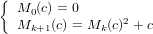
A point c belongs to the Mandelbrot set if and only if:

The following program, which uses the ParallelForPipeReduce pattern for both
computing the set line by line (Map part) and for displaying the line just computed
(Reduce part), displays the Mandelbrot set in a X window. The result is shown in
Fig 4.1.
1/* ************************ */ 2/* ******* mandel.cpp ***** */ 3 4#include <iostream> 5#include <cstdio> 6#include <cmath> 7#include <cassert> 8#include <ff/utils.hpp> 9#define HAS_CXX11_VARIADIC_TEMPLATES 1 10#include <ff/parallel_for.hpp> 11#include ”lib/marX2.h” 12 13const int DIM=800; // default dimension 14const int ITERATION=1024; // default iteration 15const double init_a=-2.125, init_b=-1.5, range=3.0; 16using namespace ff; 17 18// task type 19struct ostream_t { 20 ostream_t(const int dim):M(dim),line(-1) {} 21 std::vector<unsigned char> M; 22 int line; 23}; 24int main(int argc, char **argv) { 25 int dim = DIM, niter = ITERATION, retries=1, nworkers, chunk=0; 26 bool scheduler = true; 27 if (argc<3) { 28 printf(”\nUsage: %s <nworkers> <size> [niterations=1024]” 29 ” [retries=1] [chunk=0] [0|1]\n\n\n”, argv[0]); 30 return -1; 31 } 32 nworkers = atoi(argv[1]); 33 dim = atoi(argv[2]); 34 if (argc>=4) niter = atoi(argv[3]); 35 if (argc>=5) retries = atoi(argv[4]); 36 if (argc>=6) chunk = atoi(argv[5]); 37 if (argc>=7) scheduler = atoi(argv[6]); 38 double step = range/((double) dim); 39 double runs[retries]; 40 41 SetupXWindows(dim,dim,1,NULL,”ParallelForPipeReduce Mandelbrot”); 42 43 ParallelForPipeReduce<ostream_t*> pfr(nworkers,true); 44 45 if (scheduler) pfr.disableScheduler(false); 46 // map lambda 47 auto Map = [&](const long start, const long stop, 48 const int thid, ff_buffernode &node) { 49 for(int i=start;i<stop;i++) { 50 double im=init_b+(step*i); 51 ostream_t *task=new ostream_t(dim); 52 for (int j=0;j<dim;j++) { 53 double a=init_a+step*j; 54 double b=im; 55 const double cr = a; 56 int k=0; 57 for ( ; k<niter;k++) { 58 const double a2=a*a; 59 const double b2=b*b; 60 if ((a2+b2)>4.0) break; 61 b=2*a*b+im; 62 a=a2-b2+cr; 63 } 64 task->M[j]= (unsigned char) 255-((k*255/niter)); 65 } 66 task->line = i; 67 node.put(task); 68 } 69 }; 70 // reduce lambda 71 auto Reduce = [&](ostream_t *task) { 72 ShowLine(task->M.data(),task->M.size(),task->line); 73 delete task; 74 }; 75 double avg=0.0, var=0.0; 76 for (int r=0;r<retries;r++) { 77 ffTime(START_TIME); 78 pfr.parallel_reduce_idx(0,dim,1,chunk,Map,Reduce); 79 ffTime(STOP_TIME); 80 81 avg += runs[r] = ffTime(GET_TIME); 82 std::cout << ”Run [” << r << ”] done, time = ” << runs[r] << ”\n”; 83 } 84 avg = avg / (double) retries; 85 for (int r=0;r<retries;r++) 86 var += (runs[r] - avg) * (runs[r] - avg); 87 var /= retries; 88 std::cout << ”The average time (ms) on ” << retries 89 << ” experiments is ” << avg 90 << ” Std. Dev. is ” << sqrt(var) << ”\n”; 91 92 std::cout << ”Press a button to close the windows\n”; 93 getchar(); 94 CloseXWindows(); 95 return 0; 96}
4.3.4 Sobel filter
Let’s consider a very simple usage example in which the ff_map is used as pipeline
stage for computing the Sobel filter (see Fig. 4.2) on a stream of input images. The first
stage reads image from disk, allocates memory and then sends a task to the second
stage (the Map one) which computes the Sobel filter in parallel using a parallel-for.
Finally the image is written into the local disk. In the following code we used
OpenCV
for reading and writing images and for converting them to grayscale.
1/* ************************* */ 2/* ******* ffsobel.cpp ***** */ 3#include<iostream> 4#include<cmath> 5#include<opencv2/imgproc/imgproc.hpp> 6#include<opencv2/highgui/highgui.hpp> 7#define HAS_CXX11_VARIADIC_TEMPLATES 1 8#include <ff/pipeline.hpp> 9#include <ff/map.hpp> 10using namespace ff; 11using namespace cv; 12const int MAPWORKERS=2; 13/* my task */ 14struct Task { 15 Task(uchar *src, uchar *dst, long rows, long cols, const std::string &name): 16 src(src),dst(dst),rows(rows), cols(cols), name(name) {}; 17 uchar *src, *dst; 18 long rows, cols; 19 const std::string name; 20}; 21/* ----- utility function ------- */ 22template<typename T> 23T *Mat2uchar(cv::Mat &in) { 24 T *out = new T[in.rows * in.cols]; 25 for (int i = 0; i < in.rows; ++i) 26 for (int j = 0; j < in.cols; ++j) 27 out[i * (in.cols) + j] = in.at<T>(i, j); 28 return out; 29} 30char* getOption(char **begin, char **end, const std::string &option) { 31 char **itr = std::find(begin, end, option); 32 if (itr != end && ++itr != end) return *itr; 33 return nullptr; 34} 35#define XY2I(Y,X,COLS) (((Y) * (COLS)) + (X)) 36/* ------------------------------ */ 37// returns the gradient in the x direction 38static inline long xGradient(uchar * image, long cols, long x, long y) { 39 return image[XY2I(y-1, x-1, cols)] + 40 2*image[XY2I(y, x-1, cols)] + 41 image[XY2I(y+1, x-1, cols)] - 42 image[XY2I(y-1, x+1, cols)] - 43 2*image[XY2I(y, x+1, cols)] - 44 image[XY2I(y+1, x+1, cols)]; 45} 46// returns the gradient in the y direction 47static inline long yGradient(uchar * image, long cols, long x, long y) { 48 return image[XY2I(y-1, x-1, cols)] + 49 2*image[XY2I(y-1, x, cols)] + 50 image[XY2I(y-1, x+1, cols)] - 51 image[XY2I(y+1, x-1, cols)] - 52 2*image[XY2I(y+1, x, cols)] - 53 image[XY2I(y+1, x+1, cols)]; 54} 55// 1st stage 56struct Read: ff_node_t<Task> { 57 Read(char **images, const long num_images): 58 images((const char**)images),num_images(num_images) {} 59 60 Task *svc(Task *) { 61 for(long i=0; i<num_images; ++i) { 62 const std::string &filepath(images[i]); 63 std::string filename; 64 65 // get only the filename 66 int n=filepath.find_last_of(”/”); 67 if (n>0) filename = filepath.substr(n+1); 68 else filename = filepath; 69 70 Mat *src = new Mat; 71 *src = imread(filepath, CV_LOAD_IMAGE_GRAYSCALE); 72 if ( !src->data ) { 73 error(”reading image file %s, going on....\n”, 74 filepath.c_str()); 75 delete src; 76 continue; 77 } 78 uchar * dst = new uchar[src->rows * src->cols]; 79 for(long y = 0; y < src->rows; y++) 80 for(long x = 0; x < src->cols; x++) { 81 dst[y * src->cols + x] = 0; 82 } 83 Task *t=new Task(Mat2uchar<uchar>(*src),dst,src->rows,src->cols,filename); 84 ff_send_out(t); // sends the task t to the next stage 85 } 86 return EOS; // computation completed 87 } 88 const char **images; 89 const long num_images; 90}; 91// 2nd stage 92struct SobelStage: ff_Map<Task> { 93 // sets the maximum n. of worker for the Map 94 // spinWait is set to true 95 // the scheduler is disabled by default 96 int nw; 97 SobelStage(int mapworkers) 98 :ff_Map<Task>(mapworkers,true) {nw=mapworkers;} 99 100 Task *svc(Task *task) { 101 uchar * src = task->src, * dst = task->dst; 102 long cols = task->cols; 103 ff_Map<Task>::parallel_for(1,task->rows-1,[src,cols,&dst](const long y) { 104 for(long x = 1; x < cols - 1; x++){ 105 const long gx = xGradient(src, cols, x, y); 106 const long gy = yGradient(src, cols, x, y); 107 // approximation of sqrt(gx*gx+gy*gy) 108 long sum = abs(gx) + abs(gy); 109 if (sum > 255) sum = 255; 110 else if (sum < 0) sum = 0; 111 dst[y*cols+x] = sum; 112 } 113 }); 114 const std::string &outfile = ”./out/” + task->name; 115 imwrite(outfile, cv::Mat(task->rows, task->cols, CV_8U, dst, cv::Mat::AUTO_STEP)); 116 delete task->src; delete [] task->dst; delete task; 117 return GO_ON; 118 }; 119}; 120 121int main(int argc, char *argv[]) { 122 if (argc < 2) { 123 std::cerr << ”\nuse: ” << argv[0] 124 << ” [-m <Wrks=2>] <image-file> [image-file]\n”; 125 std::cerr << ” Wrks2 is the n. of map’s workers\n\n”; 126 return -1; 127 } 128 int start = 1; 129 int Wrks = MAPWORKERS; 130 char *m = getOption(argv, argv+argc, ”-m”); 131 if (m) { Wrks = atoi(m); start+=2; argc-=2; } 132 long num_images = argc-1; 133 assert(num_images >= 1); 134 135 Read reader(&argv[start], num_images); 136 SobelStage sobel(Wrks); 137 ff_Pipe<> pipe(reader, sobel); 138 if (pipe.run_and_wait_end()<0) { 139 error(”running pipeline\n”); 140 return -1; 141 } 142 return 0; 143}
Chapter 5
Data-flow parallelism
The data-flow programming model is a general approach to parallelization based
upon data dependencies among a program’s operations. Its theoretical and
methodological value is quite fundamental in parallel processing.
The computations is expressed by the data-flow graph, i.e. a DAG whose nodes
are instructions and arcs are pure data dependencies.
If instead of simple instructions, portions of code (sets of instructions or
functions) are used as graph’s nodes, then it is called the macro data-flow model
(MDF). The resulting MDF program is therefore represented as a graph whose nodes
are computational kernels and arcs read-after-write dependencies. It is worth noting
that, the data-flow programming model is able to work both on stream of values and
on a single value. For this reason, it is considered somehow a primitive model of
computation.
5.1 The ff_mdf data-flow skeleton
The mdf skeleton in FastFlow called ff_mdf implements the macro data-flow
parallel pattern. The run-time of the FastFlow mdf pattern is responsible for
scheduling fireable instructions (i.e. those with all input data dependencies ready)
and managing data dependencies.
Currently, the internal implementation of the FastFlow mdf pattern is a 2-stage
pipeline, the first stage is responsible for dynamically generating the graph
instructions by executing the users’ code, and the second stage (a task-farm with
feedback channel) is responsible for managing task dependencies and task scheduling.
In the next version of FastFlow, other different implementations using less resources
will be provided to the users.
ff_mdf run-time components:
At the general level, it is possible to identify the following main parts of the FastFlow mdf
run-time:
- Dynamic construction of the task graph (DAG): in complex program the task
graph could be very large; its generation time can affect significantly the
computation time, and the memory required to store the entire graph may be
extremely large. To overcome these issues, a solution is to generate the graph
during the computation of tasks (and possibly overlap task generation and task
computation), such that only a window of the graph is maintained in memory.
- Handling inter-task dependencies: Handling task dependencies, i.e. update
dependencies after the completion of previously scheduled tasks and determining
ready (fireable) tasks to be executed.
- Scheduling of fireable tasks: a task having all input dependencies ready may be
selected by the interpreter for execution. This selection needs to be performed in a
smart way in order to optimise cache locality, particular important on shared-cache
multi-core, and at the same time trying to maintain a good load balancing among
worker threads.
Creating graph tasks
In order to show how to use the mdf pattern, let’s take a look at the following simple
case. Suppose you have the following sequential code:
1const size_t SIZE = 1<<20; 2long *A,*B,*C,*D; 3allocate(A,B,C,D, size); 4sum2(A,B,SIZE); // executes A = A + B; 5sum2(C,B,SIZE); // executes C = C + B; 6sum2(D,B,SIZE); // executes D = D + B; 7sum3(D,A,C,SIZE);// executes D = A + C + D;
here we can identify 4 macro instructions that can be executed concurrently with the
FastFlow mdf pattern by specifying, for each instruction, which are the input or
output parameters of the function that has to be executed (in this case sum2
and sum3). For example, the first instruction in the code above has two
input parameters (A and B) and one output parameter (C) that have to be
passed to the function sum2. A parameter is provided to the run-time as
param_info type, which has two fields, one is the pointer of the input
or output of the ”real” parameter and the second is the ”direction” which
can be INPUT,OUTPUT or VALUE (this last one is used mainly for those
parameters that can be evaluated as a single value, do not constitute a real
dependency). The function and the parameters are passed to the run-time using
the AddTask method of the mdf class. The resulting code is the following
one:
1/* *************************** */ 2/* ******* hello_mdf.cpp ***** */ 3 4/* ________ 5 * / \ 6 * | \ 7 * A = A + B; // sum2 A B C | D 8 * C = C + B; // sum2 | | | | | 9 * D = D + B; // sum2 \ / \ / \ / 10 * D = A + C + D; // sum3 + + + 11 * A C D 12 * | | | 13 * \ \ / 14 * ----- + ----- 15 * D 16 */ 17#include <ff/mdf.hpp> 18using namespace ff; 19const size_t SIZE = 1<<8; //1<<20; 20void sum2(long *X, long *Y, const long size); 21void sum3(long *X, long *Y, long *Z, const long size); 22template<typename T> 23struct Parameters { 24 long *A,*B,*C,*D; 25 T* mdf; 26}; 27void taskGen(Parameters<ff_mdf > *const P){ 28 long *A = P->A; long *B = P->B; 29 long *C = P->C; long *D = P->D; 30 auto mdf = P->mdf; 31 32 std::vector<param_info> Param; 33 // A = A + B; 34 { 35 const param_info _1={(uintptr_t)A,INPUT}; // 1st param 36 const param_info _2={(uintptr_t)B,INPUT}; // 2nd param 37 const param_info _3={(uintptr_t)A,OUTPUT}; // 3rd param 38 // pack the parameters in one single vector 39 Param.push_back(_1); Param.push_back(_2); 40 Param.push_back(_3); 41 mdf->AddTask(Param, sum2, A,B,SIZE); // create on task 42 } 43 // C = C + B; 44 { 45 Param.clear(); 46 const param_info _1={(uintptr_t)C,INPUT}; 47 const param_info _2={(uintptr_t)B,INPUT}; 48 const param_info _3={(uintptr_t)C,OUTPUT}; 49 Param.push_back(_1); Param.push_back(_2); Param.push_back(_3); 50 mdf->AddTask(Param, sum2, C,B,SIZE); 51 } 52 // D = D + B; 53 { 54 Param.clear(); 55 const param_info _1={(uintptr_t)D,INPUT}; 56 const param_info _2={(uintptr_t)B,INPUT}; 57 const param_info _3={(uintptr_t)D,OUTPUT}; 58 Param.push_back(_1); Param.push_back(_2); Param.push_back(_3); 59 mdf->AddTask(Param, sum2, D,B,SIZE); 60 } 61 // D = A + C + D; 62 { 63 Param.clear(); 64 const param_info _1={(uintptr_t)A,INPUT}; 65 const param_info _2={(uintptr_t)C,INPUT}; 66 const param_info _3={(uintptr_t)D,INPUT}; 67 const param_info _4={(uintptr_t)D,OUTPUT}; 68 Param.push_back(_1); Param.push_back(_2); 69 Param.push_back(_3); Param.push_back(_4); 70 mdf->AddTask(Param, sum3, D,A,C,SIZE); 71 } 72} 73int main() { 74 long *A= new long[SIZE], *B= new long[SIZE]; 75 long *C= new long[SIZE], *D= new long[SIZE]; 76 for(size_t i=0;i<SIZE;++i) { 77 A[i]=i; B[i]=i+1; C[i]=i+2; D[i]=i+3; 78 } 79 // creates the mdf object passing the task generetor function 80 Parameters<ff_mdf > P; 81 ff_mdf dag(taskGen, &P); 82 P.A=A,P.B=B,P.C=C,P.D=D,P.mdf=&dag; 83 84 if (dag.run_and_wait_end() <0) error(”running dag”); 85 return 0; 86}
5.2 Examples
In this section we propose two numerical application: the block-based matrix
multiplication and the block-based Cholesky factorisation.
5.2.1 Block-based matrix multiplication
As a more complex usage example of the FastFlow mdf pattern we consider here the
block-based matrix multiplication algorithm. The algorithm is sketched in
Fig. 5.2.
This version computes in parallel the Cij blocks doing p-passes. A more
cache-friendly implementation can be implemented.
1/* ******************************** */ 2/* ******* blk_matmul_mdf.cpp ***** */ 3 4#include <assert.h> 5#include <math.h> 6#include <stdio.h> 7#include <stdlib.h> 8#include <string.h> 9#include <sys/time.h> 10 11#include <ff/mdf.hpp> 12#include <ff/parallel_for.hpp> 13using namespace ff; 14 15const double THRESHOLD = 0.001; 16bool PFSPINWAIT=false; // enable/disable spinWait 17int PFWORKERS=1; // parallel_for parallelism degree 18int PFGRAIN =0; // default static scheduling of iterations 19 20void random_init (long M, long N, long P, double *A, double *B); 21long parse_arg(const char *string); 22void printarray(const double *A, long m, long n, long N); 23// executes the standard ijk algorithm on a single block 24// using the ParallelFor pattern. This is the macro instruction. 25void blockMM(long b, const double *A, const long AN, 26 const double *B, const long BN, 27 double *C, const long CN) { 28 29 ParallelFor pf(PFWORKERS,PFSPINWAIT); 30 pf.disableScheduler(true); // removes the scheduler thread 31 pf.parallel_for(0,b,1,PFGRAIN,[A,B,AN,BN,CN,b,&C](const long i) { 32 for (long j = 0; j < b; j++) { 33 for (long k = 0; k < b; k++) 34 C[i*CN+j] += A[i*AN+k]*B[k*BN+j]; 35 } 36 }); 37} 38// put the block pointed by C to zero 39void zerosBlock(long b, double *C, const long CN) { 40 for (long i = 0; i < b; i++) 41 for (long j = 0; j < b; j++) 42 C[i*CN+j] = 0.0; 43} 44// taskGen’s parameters data type 45template<typename T> 46struct Parameters { 47 Parameters(const double *A, const double *B, double *C):A(A),B(B),C(C) {} 48 const double *A,*B; 49 double *C; 50 long AN,BN,CN; // stride 51 long b, m, n, p; // size 52 T* mdf; 53}; 54 55// Block-based algorithm: 56void taskGen(Parameters<ff_mdf > *const P){ 57 const double *A = P->A, *B = P->B; 58 double *C = P->C; 59 long m=P->m,n=P->n,p=P->p,b=P->b; 60 long AN=P->AN,BN=P->BN,CN=P->CN; 61 long mblocks = m/b, nblocks = n/b, pblocks = p/b; 62 auto mdf = P->mdf; 63 64 // set C blocks to zero 65 for(long i=0; i<mblocks; ++i) { 66 for(long j=0; j<nblocks; ++j) { 67 double *Cij = &C[b*(i*CN+j)]; 68 std::vector<param_info> Param; 69 const param_info _1={(uintptr_t)Cij, INPUT}; 70 const param_info _2={(uintptr_t)Cij, OUTPUT}; 71 Param.push_back(_1); Param.push_back(_2); 72 // create a task 73 mdf->AddTask(Param, zerosBlock, b, Cij, CN); 74 } 75 } 76 for(long k=0; k<pblocks; ++k) { 77 for(long i=0; i<mblocks; ++i) { 78 for(long j=0; j<nblocks; ++j) { 79 const double *Aik = &A[b*(i*AN + k)]; 80 const double *Bkj = &B[b*(k*BN + j)]; 81 double *Cij = &C[b*(i*CN+j)]; 82 std::vector<param_info> Param; 83 const param_info _1={(uintptr_t)Aik, INPUT}; 84 const param_info _2={(uintptr_t)Bkj, INPUT}; 85 const param_info _3={(uintptr_t)Cij, OUTPUT}; 86 Param.push_back(_1); Param.push_back(_2); Param.push_back(_3); 87 // create a task 88 mdf->AddTask(Param, blockMM, b, Aik, AN, Bkj, BN, Cij, CN); 89 } 90 } 91 } 92} 93 94int main(int argc, char* argv[]) { 95 if (argc < 5) { 96 printf(”\n\tuse: %s <M> <N> <P> <blocksize>’’ 97 printf’’ [nworkers] [pfworkers:pfgrain]\n”, argv[0]); 98 printf(”\t <-> required argument, [-] optional argument\n”); 99 printf(”\t A is M by P\n”); 100 printf(”\t B is P by N\n”); 101 printf(”\t nworkers is the n. of workers of the mdf pattern\n”); 102 printf(”\t pfworkers is the n. of workers of the ParallelFor pattern\n”); 103 printf(”\t pfgrain is the ParallelFor grain size\n”); 104 printf(”\t NOTE: the blocksize must evenly divide M, N and P.\n”); 105 return -1; 106 } 107 int nw = -1; 108 long M = parse_arg(argv[1]); 109 long N = parse_arg(argv[2]); 110 long P = parse_arg(argv[3]); 111 long b = parse_arg(argv[4]); 112 if (argc >= 6) nw = atoi(argv[5]); 113 if (argc >= 7) { 114 std::string pfarg(argv[6]); 115 int n = pfarg.find_first_of(”:”); 116 if (n>0) { 117 PFWORKERS = atoi(pfarg.substr(0,n).c_str()); 118 PFGRAIN = atoi(pfarg.substr(n+1).c_str()); 119 } else PFWORKERS = atoi(argv[6]); 120 } 121 const double *A = (double*)malloc(M*P*sizeof(double)); 122 const double *B = (double*)malloc(P*N*sizeof(double)); 123 assert(A); assert(B); 124 125 random_init(M, N, P, const_cast<double*>(A), const_cast<double*>(B)); 126 double *C = (double*)malloc(M*N*sizeof(double)); 127 128 Parameters<ff_mdf > Param(A,B,C); 129 ff_mdf mdf(taskGen, &Param,32,(nw<=0?ff_realNumCores():nw)); 130 Param.m=M,Param.n=N,Param.p=P,Param.b=b; 131 Param.AN=P,Param.BN=N,Param.CN=N; 132 Param.mdf=&mdf; 133 printf(”Executing %-40s”, ”Block-based MM”); 134 ffTime(START_TIME); 135 mdf.run_and_wait_end(); 136 ffTime(STOP_TIME); 137 printf(” Done in %11.6f secs.\n”, (ffTime(GET_TIME)/1000.0)); 138 139 free((void*)A); free((void*)B); free(C); 140 return 0; 141}
5.2.2 Block-based Cholesky factorisation
To be added
Chapter 6
Task parallelism
TBA
ff_taskf
Chapter 7
Targeting GPUs
TBA
Chapter 8
Targeting Distributed Systems
TBA
Bibliography
[1] Marco Aldinucci, Andrea Bracciali, Pietro Liò, Anil Sorathiya, and
Massimo Torquati. StochKit-FF: Efficient systems biology on multicore
architectures. In M. R. Guarracino, F. Vivien, J. L. Träff, M. Cannataro,
M. Danelutto, A. Hast, F. Perla, A. Knüpfer, B. Di Martino, and
M. Alexander, editors, Euro-Par 2010 Workshops, Proc. of the 1st
Workshop on High Performance Bioinformatics and Biomedicine (HiBB),
volume 6586 of LNCS, pages 167–175, Ischia, Italy, aug 2011. Springer.
[2] Marco Aldinucci, Marco Danelutto, Lorenzo Anardu, Massimo
Torquati, and Peter Kilpatrick. Parallel patterns + macro data flow
for multi-core programming. In Proc. of Intl. Euromicro PDP 2012:
Parallel Distributed and network-based Processing, pages 27–36, Garching,
Germany, feb 2012. IEEE.
[3] Marco Aldinucci, Marco Danelutto, Peter Kilpatrick, Massimiliano
Meneghin, and Massimo Torquati. Accelerating sequential programs using
FastFlow and self-offloading. Technical Report TR-10-03, Università di
Pisa, Dipartimento di Informatica, Italy, feb 2010.
[4] Marco Aldinucci, Marco Danelutto, Peter Kilpatrick, Massimiliano
Meneghin, and Massimo Torquati. Accelerating code on multi-cores with
fastflow. In E. Jeannot, R. Namyst, and J. Roman, editors, Proc. of
17th Intl. Euro-Par 2011 Parallel Processing, volume 6853 of LNCS, pages
170–181, Bordeaux, France, August 2011. Springer.
[5] Marco Aldinucci, Marco Danelutto, Peter Kilpatrick, and Massimo
Torquati. Fastflow: high-level and efficient streaming on multi-core. In Sabri
Pllana and Fatos Xhafa, editors, Programming Multi-core and Many-core
Computing Systems, Parallel and Distributed Computing, chapter 13.
Wiley, March 2014.
[6] Marco Aldinucci, Marco Danelutto, Massimiliano Meneghin, Peter
Kilpatrick, and Massimo Torquati. Efficient streaming applications on
multi-core with FastFlow: the biosequence alignment test-bed. In Barbara
Chapman, Frédéric Desprez, Gerhard R. Joubert, Alain Lichnewsky, Frans
Peters, and Thierry Priol, editors, Parallel Computing: From Multicores
and GPU’s to Petascale (Proc. of PARCO 2009, Lyon, France), volume 19
of Advances in Parallel Computing, pages 273–280, Lyon, France, 2010. IOS
press.
[7] Marco Aldinucci, Massimiliano Meneghin, and Massimo Torquati.
Efficient Smith-Waterman on multi-core with fastflow. In Marco Danelutto,
Tom Gross, and Julien Bourgeois, editors, Proc. of Intl. Euromicro PDP
2010: Parallel Distributed and network-based Processing, pages 195–199,
Pisa, Italy, feb 2010. IEEE.
[8] Marco Aldinucci, Salvatore Ruggieri, and Massimo Torquati. Decision
tree building on multi-core using fastflow. Concurrency and Computation:
Practice and Experience, 26(3):800–820, March 2014.
[9] Marco Aldinucci and Massimo Torquati. FastFlow website, 2009.
http://mc-_fastflow.sourceforge.net/.
[10] Marco Aldinucci, Massimo Torquati, and Massimiliano Meneghin.
FastFlow: Efficient parallel streaming applications on multi-core. Technical
Report TR-09-12, Università di Pisa, Dipartimento di Informatica, Italy,
sep 2009.
[11] Marco Aldinucci, Massimo Torquati, Concetto Spampinato, Maurizio
Drocco, Claudia Misale, Cristina Calcagno, and Mario Coppo. Parallel
stochastic systems biology in the cloud. Briefings in Bioinformatics, June
2013.
[12] Murray Cole. Algorithmic Skeletons: Structured Management of
Parallel Computations. Research Monographs in Par. and Distrib.
Computing. Pitman, 1989.
[13] Murray Cole. Bringing skeletons out of the closet: A pragmatic
manifesto for skeletal parallel programming. Parallel Computing,
30(3):389–406, 2004.
[14] Marco Danelutto. Distributed Systems: Paradigms and Models. SPM
cource note, Computer Science Department University of Pisa, 2013.
[15] Marco Danelutto, Luca Deri, Daniele De Sensi, and Massimo Torquati.
Deep packet inspection on commodity hardware using fastflow. In Proc. of
PARCO 2013 Conference, Munich, Germany, Munich, Germany, 2013.
[16] Marco Danelutto and Massimo Torquati. Structured parallel
programming with ”core” fastflow. In Formal Methods for Components
and Objects: 7th Intl. Symposium, FMCO 2008, Sophia-Antipolis, France,
October 20 - 24, 2008, Revised Lectures, volume 8606 of LNCS, pages 28–74.
Springer, 2014.
[17] Horacio González-Vélez and Mario Leyton. A survey of algorithmic
skeleton frameworks: high-level structured parallel programming enablers.
Softw., Pract. Exper., 40(12):1135–1160, 2010.
[18] Claudia Misale, Giulio Ferrero, Massimo Torquati, and Marco
Aldinucci. Sequence alignment tools: one parallel pattern to rule them all?
BioMed Research International, 2014.